
Grid-forming (GFM) technology is one of the latest hot topics in power systems, and for good reason. Although it isn’t technically new, modern applications of GFM technology are showing incredible potential for solving some of the most difficult problems we face in power systems with high shares of inverter-based resources (IBRs). GFM controls can provide weak-grid stabilization, extremely fast and effective frequency response, and damping of sub-synchronous oscillations, all while providing the basic grid-control functions required of all generation resources.

When simulating GFM in power systems with high shares of IBRs, from a pure modeling standpoint the basic approach is no different than simulating conventional systems. At the present time, models in both the phasor and electro-magnetic transient (EMT) domains are being developed to simulate GFM, and both types of tools will remain important going forward. However, since many of the recent industrial applications of GFM are exploring brand new controls with relatively untested hardware, this blog post is focused on the more detailed EMT side that is our specialty at Electranix. We are not focused here on what EMT is, why we do it, or when it needs to be done. This is no longer new, and is now a routine part of our work. Numerous electric utilities around the world are now conducting EMT studies as a routine part of their interconnection planning, and there is a large body of literature and guidance, as well as requirements and standards which inform us that EMT will be a part of our lives going forward. What we’ll touch on here is the how.
How Do We Simulate Power Systems with High Shares of GFM IBR Resources?
In brief, we’ll outline how we at Electranix are approaching the task of modeling high penetration systems in EMT, including the most recent GFM technology. We model renewable saturated systems large and small, looking for interconnection and operation issues such as control interactions, ride-through failure, and weak system instabilities that may be hard to catch using conventional RMS tools. This is our specialty, and we think we do it well, but I will happily recognize that there are lots of experts out there, and we’re all exploring ways to do it better! For us, it goes roughly as follows:
-
- Recognize that there are constraints on the tools and on our time. We use powerful computers, but the simulations still run slowly, and take a lot of time. We can’t study everything we’d like to, so we need to go into each study consciously focusing our efforts and sharpening the questions we need answered.
- Work collaboratively to carefully define the scope, including study boundaries (including which devices are important to model) and key scenarios and outages. Decide which elements of the system are relevant to the analysis you’re doing, such as frequency dependent lines, transformer saturation, special protection elements, etc. There is a significant amount of work in this step, but doing it well allows the overall process to be more effective.
- Collect models and test each one individually for quality and compliance with pre-defined model accuracy criteria. We have our own standard, as do many utilities, and this is also coming to more formal processes through efforts like IEEE 2800.2.
- All models are containerized and organized into a standard library format for input into our E-Tran conversion tool and for ease of re-use in future studies. This minimizes re-work and errors in model construction.
- Starting with solved power flow cases which represent the scenarios we want to study, we build parallelized system models using E-Tran and E-Tran Plus tools. These tools do a lot of the grunt modeling work for us, including modeling of multi-port system equivalents for the system outside our study boundary, automation of key contingencies, configuring monitoring logic to see key power system quantities, and even automatic “expert system” analysis if required.
- We perform preliminary runs and checks on the system model and contingencies, finalizing monitoring automation and doing sanity checks on contingency automation.
- Analysis and mitigation iterations are performed until the overall system is able to perform acceptably.
What Should We Expect to See?
For GFM applications in particular, it is important during the analysis phase to adapt our understanding of what we should expect. Just as we needed to adapt our “analysis reflexes” to understand conventional grid-following (GFL) IBR behavior, when our eyes were used to seeing synchronous machine responses, so we need to adapt again to understand what a GFM behavior can and should look like in a system context. For example, Figure 1 shows that loss of a generator unit in the system causes the remaining generators to respond with frequency controls in different ways. We are used to the black and red traces (synchronous generators and GFL IBRs), but a GFM battery can be designed to respond in new and powerful ways. We need to understand the performance we want, ask for it, and look for that performance in our analysis.
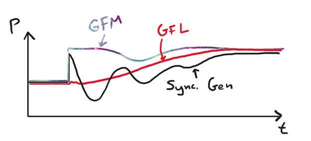
Figure 1. A GFL battery, a GFM battery, and a synchronous generator can all respond to a loss of nearby generator in different ways.
What Are We Waiting for?
As we start to unlock the capabilities of GFM technology, we will gain more experience and practice with this. GFM controls coming out of manufacturers’ research and development skunkworks are still changing as they optimize and tune GFM IBR behavior according to what the studies and fresh industry experience are telling them they need to do. As we learn from early adoption, simulation, and studies, we become more confident in writing requirements and standards to help manufacturers sharpen their product offerings, compete effectively, and reduce cost.
We shouldn’t wait. The study capability is available, the GFM technology is available, and the need for powerful devices to smooth the accelerating transition to renewable energy is certainly here already. Many gigawatts of batteries are currently connecting or are being planned to connect to our grids in the next few years. This is low-hanging fruit, so let’s start building these batteries GFM now!
Andrew Isaacs
Vice President, Electranix