Formulating a Simplified Equivalent Representation of Distribution Circuits for PV Impact Studies

Author: Sandia National Laboratories^[1]

With an increasing number of Distributed Generation (DG) being connected on the distribution system, a method for simplifying the complexity of the distribution system to an equivalent representation of the feeder is advantageous for streamlining the interconnection study process. The general characteristics of the system can be retained while reducing the modeling effort required. This report presents a method of simplifying feeders to only specified buses-of-interest. These buses-of-interest can be potential PV interconnection locations or buses where engineers want to verify a certain power quality. The equations and methodology are presented with mathematical proofs of the equivalence of the circuit reduction method. An example 15-bus feeder is shown with the parameters and intermediate example reduction steps to simplify the circuit to 4 buses. The reduced feeder is simulated using PowerWorld Simulator to validate that those buses operate with the same characteristics as the original circuit. Validation of the method is also performed for snapshot and time-series simulations with variable load and solar energy output data to validate the equivalent performance of the reduced circuit with the interconnection of PV.

Introduction

With an increasing number of Distributed Generation (DG) being connected on the distribution system, a method for simplifying the complexity of the distribution system to an equivalent representation of the feeder is advantageous for streamlining the interconnection study process. Interconnection studies are required to study the impacts of high deployment levels of PV on a distribution system when the PV levels exceed screening thresholds for fast track approval^[2]. A full detailed model of the distribution system can be time consuming to produce, and a time-series simulation of a large system at a high time-resolution requires significant computational processing^[3][4][5]. A simplified equivalent circuit will retain the general characteristics of the distribution system and will also reduce the modeling effort required.

This paper describes an analytical approach that can be used to derive the simplified equivalent representation of the circuit. A distribution feeder, which will typically have hundreds to thousands of line sections and nodes, can be simplified to an equivalent circuit with far fewer line sections and nodes. The reduced circuit maintains the feeder topology and characteristics so that it performs the same in simulation. This representation also preserves any specific buses where voltage or other performance measures are important. These specific buses, or buses-of-interest, represent critical points in the circuit, including: voltage regulation equipment locations, potential PV point of common coupling (PCC) interconnection locations, or extreme voltage locations on the feeder. The number of buses in the simplified circuit depends on how many buses-of-interest are selected (n), plus some buses-of-interest to represent the topology of the distribution system. The final reduced circuit will contain between n and 2*n, with no more than twice the selected buses-of-interest in the reduced circuit. For example, a distribution feeder with 6 capacitor banks and 4 voltage regulators would reduce to less than 20 buses, independent of the number of loads or the length of the feeder. The buses-of-interest are retained in the reduced circuit maintaining equivalent performance as the full circuit, and all other circuit details are simplified to the minimum amount of necessary information.

One benefit of using a simplified equivalent representation for the feeder is the ability to reduce the feeder complexity to improve the ease of converting the feeder circuit from one software or analysis package to another. Existing models are often in distribution system programs with limitations for interconnection analysis, such as the available PV models and time-series simulation capabilities of the software. With fewer line segments in the reduced circuit, it would be much simpler and faster to convert feeders from commercial power flow software packages to software like OpenDSS that is open source and can do quasi-static time-series analysis for interconnection studies. The simplified feeder can also provide faster and more accurate interconnection screening criteria by reducing the circuit to a simpler equivalent representation with only the key circuit parameters, which could be used to quickly identify the PV impact risk score for a feeder. Finally, if a full interconnection study is required for a proposed PV system, a simplified equivalent representation would decrease the simulation system size. Time-series analyses of a large distribution system with many feeders, stochastic simulations, or multiple PV study scenarios simulated at a high time-resolution require significant computational processing for full circuit models. With a reduced circuit model, the simulation could stochastically loop through many different scenarios very quickly. For detailed time-series simulation, this would decrease simulation run times, reduce required processing power, and decrease the computer memory required, while still providing the full accuracy of the full feeder model.

Background

Many methods for circuit reduction have been published for different purposes, and some examples of circuit reduction techniques can be seen in^{[8][9][10][11][12][13]}. These are often a reapplication of basic circuit analysis techniques to calculate circuit parameters for a simpler representation. One key circuit equivalencing technique that deserves special attention comes from the Western Electricity Coordinating Council (WECC) guideline for modeling wind power plants^[14]. The solar energy field has learned many things from wind advancements, and WECC published a similar guideline for modeling PV systems in large-scale power flow simulations based on the wind guideline^[6]. Both WECC guidelines use the same method for reducing the circuit, and it is well established in other literature^[15][16].

The WECC equivalencing method was first published for reducing a collector system of a large wind power plant^[17]. The method reduces a multi-machine system with varying impedances between the collector and the wind turbine generators to a single equivalent machine and single equivalent impedance representation. The single machine represents the average conditions on the wind power plant, and the single equivalent impedance is the average impedance weighed by the square of the current. This method was formulated in order to produce real and reactive line losses equivalent to the full wind power plant network. The equivalent impedance of the wind power plant is the sum of the individual line losses (current²*impedance) divided by square of the total current being produced by the wind power plant, I_total. For each line with impedance Z_m and current I_Zm, the equivalent impedance for a collector with n line segments is

\(Z_{eq} = \cfrac{\sum_{m=1}^n I_{Zm}^2 Z_m}{I_{total}^2}\)

The simplest implementation of this method assumes that all turbines have the same power output and rating, so the I_Zm terms in equation above for current can be represented by the number of downstream turbines and I_total is the total number of turbines^[17]. The more advanced method uses the actual current in the lines to allow for different turbine or inverter ratings^[18]. The WECC literature proposes a method similar to a DC power flow to calculate the line currents I_Zm in the above equation. DC power flow is commonly used in a simplified model of the power system network as a rough approximation for such tasks as production costing and trading optimization because of the speed and simplicity of the calculation due to disregarding reactive power, voltage levels, and active power losses. Since all voltages are fixed, it is a system of linear constant equations that can be solved without iteration. The WECC method can use this approximation, along with the fact that it is a radial network, to approximate I_Zm by hand without solving the full power flow or having to form the Ybus impedance matrix. It is important to remember that this method of calculating line currents is an approximation because the line losses make the assumption of equal bus voltages false, but it is not a bad approximation since the variation in voltages is small. If the simplified DC power flow is used, the equivalent impedance is slightly different than the exact equivalent impedance. When compared to the full plant representation, this simplified model varies slightly with regard to plant short-circuit contribution as well as the power angle with reference to the grid. The method provides an easy-to-calculate approximation that can be done by hand, and has been shown to work well for wind transient and stability studies^[19] and for evaluating wind farm harmonics^[20]. Errors for reactive power loss can be higher than active power errors because of the assumption that reactive power generated by the line capacitive shunts is at one per unit voltage^[17]. In^[21] it is shown that the WECC single turbine representation does not perform well under some conditions of diversity in line impedance, diversity in power production, or diversity of generation types. The WECC method allows both active and reactive losses to be approximated by hand. The approximation in the WECC method is in the calculation of I_Zm, so if higher accuracy is required, the full wind or solar plant information along with the entire collector information can be entered into a power simulation package to solve for the full power flow.

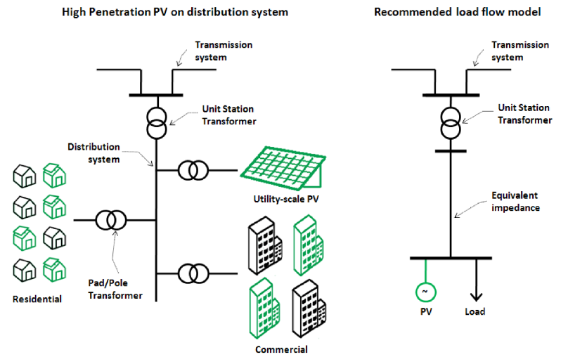
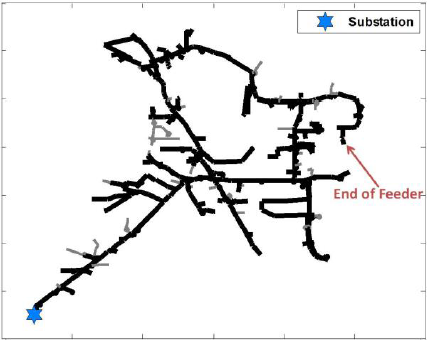
The WECC equivalencing method is designed for studying the impact of large plants on the bulk electric transmission system, and it cannot easily be used to tackle the system in figure on the right because of the diversity of loads and generators. The objectives of the WECC method did not include interest in the voltages or details inside the feeder, only their impacts on the transmission system. Once the circuit is reduced to an equivalent “average” load and “average” DG shown in figure on the right, the model does not provide any information about the voltage deviations or extreme voltages inside the distribution system that are valuable for studying the impact of DG on the distribution system. The WECC model was never intended to be applicable to this case. To study the impact of PV on the distribution system, the equivalent circuit must preserve the locational value of solar with impacts to specific parts of the feeder and correctly model voltages inside the feeder, especially at locations with voltage regulation equipment.

The WECC model is useful for quickly approximating the equivalent impedance for a singlemachine representation of a large wind power plant or a large PV plant. This could be used for modeling large central PV systems interconnected on the distribution system, but reducing the entire feeder would lose details necessary for distribution system interconnection impact studies.

Because the method assumes fixed voltage on all buses, it probably would not work well for equivalencing large distributed PV systems connected on the secondary system of the distribution system where the voltage varies significantly at locations around the feeder. The WECC equivalent impedance also requires all line currents to change in proportion to one another through time. This is a good approximation for a large wind power plant or large PV plant where all inverters in the plant increase or decrease together in time, but it is more complicated to apply to distributed rooftop solar, especially with dispersed loads in the feeder each with different load shapes through time.

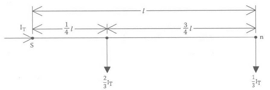
Another method called the exact lumped load model was specifically developed for reducing the complexity of loads on the distribution system^[7]. The reduced circuit model includes the extreme feeder voltages by modeling the voltage drops in the circuit. This method assumes that all loads are constant current loads and are uniformly distributed along a line in the feeder with equal spacing and equal magnitude. The uniformly distributed requirement is a big assumption and limitation of the method, but this is most commonly the case on single phase laterals where equally rated transformers are regularly spaced along the lateral. The method could also be used for large PV plants where equally rated inverters are equally spaced throughout the plant. The exact lumped load model ensures that the voltage drop to the end of the line is the same in the reduced model and that the line losses are equal. For simplification and approximation, the model is developed for the case where the number of loads goes to infinity and the distance between the loads goes to zero. With these assumptions, the resulting model for a feeder with length l and total feeder load I_T is shown in figure on the right.

The exact lumped load model is useful in specific circumstances with uniformly distributed loads, or it can provide a reasonable assumption for line losses and voltage drop along a feeder if the load sizes or locations are unknown. In contrast, if a simplified equivalent circuit for a full distribution system model is required, the exact lumped load model does not capture the diversity of line impedances and load sizes. Specific sections of the feeder may be applicable to use the exact lumped load model, but the model could not provide an equivalent representation for an entire feeder due to the complexity of load sizes (residential, industrial, commercial), range of line lengths in the feeder, and variety of possible distributed rooftop PV sizes. The load bus reduction methodology is formulated with a similar process to the exact lumped load model without the uniformly distributed loads assumption.

Load Bus Reduction Formulation

Given the limitations of the methods previously discussed, a method is developed for reducing the distribution system to an equivalent circuit for performing PV interconnection studies. The reduced circuit must keep the important details like voltage regulators in the circuit while reducing the total number of buses. A method is developed and demonstrated for load bus reduction that combines a load bus into the two adjacently connected buses, thus removing the bus from the circuit. With reduction, all bus voltages and the current going into the network remain the same. In this manner, the circuit is fully equivalent to the original circuit power flow except with fewer buses.

The load bus reduction method is based on the key assumption that all loads on the feeder are fixed current loads. This is an important deviation from many power flow simulations that assume fixed P/Q loads. See herefor more discussion of fixed current loads and evaluation of the assumption on the circuit reduction method. The reduction method also assumes balanced loads, balanced wire impedance, no shunt capacitance, and no mutual coupling. Future research will further investigate the impacts of these factors in the reduction of the circuit.

Single Load Bus Reduction

The method for load bus reduction is shown for the simplest case with 2 line sections with impedances Z₁ and Z₂ connecting three buses with load currents L₁, L₂, L₃ as shown in “Load bus reduction” figure. The L variables represent the current consumed by the fixed current loads with the units of L being in Amps. If bus 2 is unnecessary in the equivalent circuit, it can be removed by combining L₂ into L₁ and L₃, resulting in a single line section Z_eq and only two load currents L_eq1 and L_eq2. The resulting reduced circuit has the same voltages V₁ and V₂ and the same current I_s coming into the circuit.

The values for the equivalent circuit are shown in the following three equations. Note that the impedance between bus 3 and bus 1 remains the same, so all results for short circuit and protection studies are unchanged. The total circuit load current is also the same with L_eq1+L_eq2=L₁+L₂+L₃.

\(Z_{eq} = Z_1+Z_2\) \(L_{eq1} = L_1+\cfrac{Z_2}{Z_1+Z_2}L_2\) \(L_{eq2} = L_3+\cfrac{Z_1}{Z_1+Z_2}L_2\)

Equivalent Voltage Drop

These equations can be derived by equating the voltage drop between V₁ and V₃. The identical voltage drop must be identical for the full circuit and the equivalent circuit. The voltage drop for the equivalent circuit is

\(V_1-V_3 = L_{eq2}Z_{eq}\)

The voltage drop for the full circuit is shown to be the same as the equivalencing method proposed in equations (1)-(3). The voltage for the full circuit is

\(\begin{align}
V_1-V_3 & = \left (L_2+L_3\right )Z_1+\left (L_3\right )Z_2\\
& = L_3\left (Z_1+Z_2\right )+L_2Z_1\\
& = L_3\left (Z_1+Z_2\right )+L_2Z_1\cfrac{Z_1+Z_2}{Z_1+Z_2}\\
& = \left (L_3+\cfrac{Z_1}{Z_1+Z_2}L_2\right )\left (Z_1+Z_2\right )\\
& = L_{eq2}Z_{eq}\\
\end{align}\)

By using equations (1) and (3), the voltage drop is equal on the reduced circuit. In order for the current Is to be the same entering the circuit, L_eq1 and L_eq2 must equal L₁+L₂+L₃, and L_eq1 can be shown to be the difference between L₁+L₂+L₃ and L_eq2, where equation (11) is equal to the reduction method in equation (3).

\(\begin{align}
L_{eq1} & = L_1+L_2+L_3-L_{eq2}\\
& = L_1+L_2+L_3-\left (L_3+\cfrac{Z_1}{Z_1+Z_2}L_2\right )\\
& = L_1+L_2-\cfrac{Z_1}{Z_1+Z_2}L_2\\
& = L_1+\cfrac{Z_1+Z_2}{Z_1+Z_2}L_2-\cfrac{Z_1}{Z_1+Z_2}L_2\\
& = L_1+\cfrac{Z_2}{Z_1+Z_2}L_2\\
\end{align}\)

Equivalent Power with Line Losses

The derivation and formulation of the above equivalent circuit was done to produce equal voltage drop between the equivalent circuit and the full circuit. The equivalent circuit can also be shown to be fully equivalent accounting for line losses. The power consumption by the full circuit including line losses is

\(V_1L_1+Z_1\left (L_2+L_3\right )^2+V_2L_2+Z_2L_3^2+V_3L_3\)

The power consumption by the equivalent circuit including line losses is

\(V_1L_1+V_1\cfrac{Z_2}{Z_1+Z_2}L_2+\left (L_3+\cfrac{Z_1}{Z_1+Z_2}L_2\right )^2\left (Z_1+Z_2\right )+V_3\cfrac{Z_1}{Z_1+Z_2}L_2+V_3L_3\)

Using the equivalent circuit equation, by expanding the squared term in the above equation and in some instances substituting in for V₁=V₂+Z₁(L₂+L₃) and V₃=V₂-Z₂L₃, the equation is

\(\begin{align}
& = V_1L_1+\left (V_2+Z_1(L_2+L_3)\right )\cfrac{Z_2L_2}{Z_1+Z_2}+L_3^2(Z_1+Z_2)+2Z_1L_2L_3+\cfrac{Z_1^2L_2^2}{Z_1+Z_2}+(V_2-Z_2L_3)\cfrac{Z_1L_2}{Z_1+Z_2}+V_3L_3\\
& = V_1L_1+V_2L_2\left (\cfrac{Z_2}{Z_1+Z_2}+\cfrac{Z_1}{Z_1+Z_2}\right )+\cfrac{Z_1Z_2L_2^2}{Z_1+Z_2}+\cfrac{Z_1Z_2L_2L_3}{Z_1+Z_2}+L_3^2(Z_1+Z_2)+2Z_1L_2L_3+\cfrac{Z_1^2L_2^2}{Z_1+Z_2}-\cfrac{Z_1Z_2L_2L_3}{Z_1+Z_2}+V_3L_3\\
& = V_1L_1+V_2L_2+Z_1L_2^2\left (\cfrac{Z_2}{Z_1+Z_2}+\cfrac{Z_1}{Z_1+Z_2}\right )+L_3^2(Z_1+Z_2)+2Z_1L_2L_3+V_3L_3\\
& = V_1L_1+V_2L_2+\left (Z_1L_2^2+2Z_1L_2L_3+Z_1L_3^2\right )+Z_2L_3^2+V_3L_3\\
& = V_1L_1+Z_1\left (L_2+L_3\right )^2+V_2L_2+Z_2L_3^2+V_3L_3\\
\end{align}\)

Thus, the total power for the equivalent circuit, shown in equation above, is the same as the total power for the full circuit shown in equation (1). Note that while the line losses are accounted for in the equivalent model and the total power of the circuit is equal, if the line losses are directly calculated for each model, the I²R losses will be different for the current flow. By moving part of L₂ to the first bus, the line losses are included in the movement of the fixed current load to the higher voltage. The line losses will always be correct, as shown above, but the line losses associated with L₂ in the reduced circuit is the combination of additional current flow along Z_eq and the increased power consumption from placing part of the fixed current load at a slightly higher voltage V₁.

Multiple Load Bus Reduction

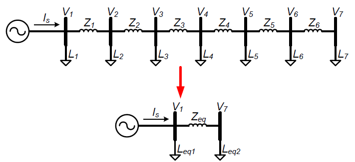
The above process for reducing a single load bus can be repeated any number of times (recursively) to combine each load current into the load currents on either side of it using equations (1)-(3). Any chain of loads can be reduced into two buses. For example, the seven load buses shown in “Multiple load bus reduction” figure can be combined into two buses (V₁ and V₇). Each fixed current load in between the buses-of-interest is combined with the load currents on either side in proportion to the line impedances.

Note that if the loads are equally spaced along the line where all line impedances between the buses are equal, equations (2) and (3) show that the reduced load bus is equally split between each adjacent bus. When the loads are equal in magnitude in addition to equally spaced, the equivalent circuit is half the load current at either end of the line section.

For any number of loads or feeder length, reducing a long section such as shown in the “Multiple load bus reduction” figure will result in half of the load current at the beginning of the line section and half of the load current at the end. The reduction of uniform loads to two equal loads at either end is also shown in^[7]. If the circuit in this figure has uniform loads with magnitude L and impedance Z between all of them, the equivalent circuit is

\(Z_{eq} = 6\times Z\) \(L_{eq1} = \cfrac{7}{2}L\) \(L_{eq2} = \cfrac{7}{2}L\)

Reduction of Branches and Preserving Feeder Topology

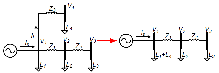
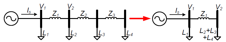
The method of load bus reduction allows any string of load buses to be combined, but realistic distribution feeders contain many branching sections and laterals. If the voltage on the branch or lateral is not required in the reduced circuit, all loads on the branch can be reduced by combining the loads onto the location of the branch split from the path that contains buses-of-interest. This is shown in the “Branches or laterals combination” figure where the equivalent load current at bus 1 is the sum of the load currents on the lateral. The method can be performed when the voltage V4 and the voltage drop between V1 and V₄ is not desired in the equivalent circuit.

The reduced circuit will have the same measured voltages at the buses-of-interest and the same current flowing into the network. The reduced circuit is fully equivalent and accounts for the line losses in Z3 because the loads are fixed current loads. For example, the L₄ load current when moved to bus 1 is connected at a slightly higher voltage bus in the distribution system. The difference in voltage between bus 1 and bus 4 is due to the line loss from the current flowing to L₄, so placing the fixed current load at the higher voltage equals the total power consumption of the original circuit for the load and the line loss. The power flowing into the lateral shows the equality of moving L₄ to V₁. In this simple case the current flowing into the lateral I_L=L₄. The total power in the lateral is

\(P = L_4*V_4+\left (L_4\right )^2Z_3\)

With some manipulation, the total power in the lateral (see above equation) is shown to equal the total power when L₄ is moved to bus 1 at V₁.

\(L_4*V_4+\left (L_4\right )^2Z_3 = L_4(V_4+L_4Z_3) = L_4V_1\)

While the total power is the same and the line losses are always fully accounted for the equivalent circuit, the line losses directly calculated using the I²R losses will be different. This is similar to the previous discussion for load bus reduction where by moving L₄, the line losses are included in the movement of the current source to the higher voltage. Line losses will always be correctly modeled in the equivalent, as shown in the two equations above, but the circuit line losses can no longer be calculated using I²R.

Any buses after a bus-of-interest can be reduced similarly to branch or lateral combination. If the voltage at the end of the lateral is not required, any bus downstream of a bus-of-interest is handled like a branch and can be combined back to the branch of interest, as shown in the “Downstream loads combined into a bus-of-interest” figure. Note that the voltage at V₂ is the same in both circuits because

\(V_2 = V_1-Z_1(L_2+L_3+L_4)\)

Preserving Feeder Topology

If there is a bus-of-interest on a branch in the feeder, the branch cannot be removed in the reduced circuit; otherwise the topology of the feeder would be modified in the equivalent circuit. The bus where the network splits must also remain if there is a bus-of-interest on each branch, but all loads on the branches can be reduced. For example, if V₃ and V₅ in the “Two buses-of-interest creating a branching equivalent circuit” figure are buses-of-interest, the circuit can be reduced to three buses and three load currents, where the three equivalent load currents are the sum of the load currents in between each bus-of-interest.

\(L_{eq1} = L_1+\cfrac{Z_2}{Z_1+Z_2}L_2+\cfrac{Z_4}{Z_3Z_4}L_4\) \(L_{eq2} = L_3+\cfrac{Z_1}{Z_1+Z_2}L_2\) \(L_{eq3} = L_5+\cfrac{Z_3}{Z_3+Z_4}L_4\)

Discussion of Fixed Current Load Assumption

The proposed circuit reduction method is based on the key assumption that all loads on the feeder are fixed current loads, and not fixed P/Q loads as is commonly the assumption for power systems analysis and power flow simulations. This section discusses the differences between the load model types used for simulations and any deviations that may be introduced by modeling loads as fixed current loads instead of fixed P/Q loads.

The load type determines the model for the power consumption as a function of the voltage. As part of their Distribution Green Circuits program, EPRI has done experimental research on distribution feeders using conservation voltage reduction (CVR), showing empirically that every 1% reduction in voltage results in an average of 0.8% reduction in real power, or a CVR=0.8%^[22]. For a fixed current load model, the power consumption is directly related to the voltage; therefore, CVR=1% for fixed current loads. Conversely, the power consumption does not change for fixed P/Q loads, which corresponds to a CVR=0%. Loads are also sometimes modeled as fixed impedance loads where the power is a function of the square of the voltage, in which case CVR=1.99%. From the point of view of power consumption as a function of voltage, modeling loads as fixed current loads is a valid assumption (CVR=1% vs. CVR=0.8% from EPRI’s Distribution Green Circuits research), and may even be more accurate than modeling loads as fixed P/Q or fixed impedance.

While the power consumption as a function of voltage depends on the load model, there is very little difference in simulation results between different load model types. During the circuit model creation, the load types are selected for the feeder, and the load allocation process tunes the simulation model results to match the measured data from the feeder. If the load measurements are taken at the substation, when the load is allocated around the feeder, the simulation results must verify that the power at the substation is still the same as measured. In this case, for a fixed current load model, no tuning will be required because the substation voltage times the sum of all the load currents will always equal the measured power at the substation. If fixed P/Q load models are used, an iterative process must be used to match the sum of power consumption of the loads and all line losses to the measured power at the substation. In the event that the feeder data provided contains load measurements at the loads instead of the substation, the two load models switch roles in their need for calibration, causing the fixed current model to require tuning while the fixed P/Q model will not. For more information on load allocation see^[7]. The load allocation process was performed for the full detail distribution feeder shown in the “Example feeder for load allocation of different load types” figure using the load measurements at the substation. The models were calibrated to match the measured real and reactive power for each phase with a total feeder load of approximately 6 MW at 0.9 power factor. Simulations were run for three load model types: fixed P/Q, fixed current, and CVR type. The “CVR load” represents the results from^[22]with CVR=0.8% for real power and CVR=3% for reactive power. The per unit phase voltages for each load type are shown in the following table.

End of feeder voltages (pu) with different load types

	Power	Current	CVR
Phase A Voltage (pu)	1.01823	1.01835	1.01843
Phase B Voltage (pu)	1.02162	1.02153	1.02150
Phase C Voltage (pu)	1.02354	1.02331	1.02320

Table below demonstrates that the simulation results for a feeder are very similar independent of the type of load model. Table below also shows that using a fixed current load model is much closer to the actual feeder response, as measured by EPRI’s CVR research.

Average percent difference for end of feeder voltages with different load type models

Current Vs. Power	Current Vs. CVR	Power Vs. CVR
0.015%	0.007%	0.022%

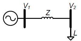
The results for the real distribution feeder model above are very small, but the theoretical maximum error will be shown using an extreme case and the simple circuit in the “Simple circuit for discussion about load model types” figure. The same three load models are investigated, and the circuits are calibrated to have the same power flow at V₁ of 1000+ j200 kVA. These extreme cases will use the full allowed voltage range 1.0±0.05 pu, with the ΔV between V₁ and V₂ equal to 0.05 pu for the base case simulation. As seen in table below, for this simple circuit, the load allocation and calibration process makes the simulation voltages equal for the different load types. For any new study scenario that would change the voltages, the percent change in the load power consumption due to the new voltage depends on the load model type. For example, simulations with new PV, different voltage control algorithms, the addition of capacitors, and expansion of existing loads will all present differences in simulation results between fixed current and fixed P/Q loads. In this case, the generator at V₁has changed the voltage setpoint from 1.0 pu to 1.05 pu and the simulation results in table below deviate between load models. Even for this extreme case, the fixed current load model is within ~0.0025 pu voltage of the fixed P/Q load model. As shown in the “Percent difference in simulation voltages for different load type models” table, the fixed current load model is much more accurate compared to the CVR voltage than fixed power loads.

Bus voltages for two scenarios with different load type models

		Power	Current	CVR
Base Case V1 setpoint=1.0	V1 (pu)	1.0	1.0	1.0
	V2 (pu)	0.95	0.95	0.95
Increased V1 setpoint=1.05	V1 (pu)	1.05	1.05	1.05
	V2 (pu)	1.0027	1	0.99974

 

Percent difference in simulation voltages for different load type models

Current Vs. Power	Current Vs. CVR	Power Vs. CVR
0.267%	-0.033%	0.300%

The load model type does not significantly impact simulation results. For a full feeder model, the simulation differences were less than 0.025% for different load models. Using an extreme case, the maximum possible error between fixed power and fixed current load models is less than 0.3%. Compared to empirical CVR research in^[22], a fixed current load model is more accurate representation of real feeders than a fixed P/Q load and would have less model error compared to average distribution system loads. Therefore, the assumption of fixed current loads does not negatively impact the circuit reduction results.

Full Feeder Reduction Method and Validation

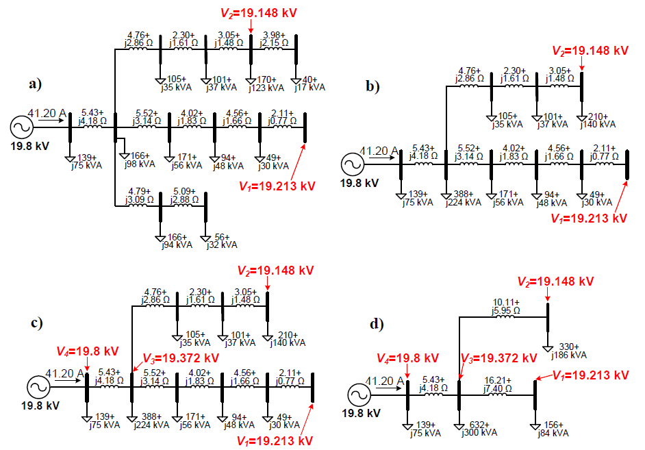
The formulation and equivalence of the circuit reduction method was shown above and is now applied to an example distribution feeder to reduce the number of buses. The example 15-bus feeder shown in the “Initial 15-bus circuit simulation” figure meets all the specified conditions and limitations of the method and is used to demonstrate the full feeder reduction method. Each step of the reduction process is explained in detail, and the equivalent circuits with all circuit parameters for each step are shown in the “Full feeder reduction method” figure.

The equivalence is validated during each step by simulating the shown circuits in PowerWorld Simulator to solve the power flow for voltages and currents. In the figures, voltages are line to line, current is per phase, and impedances are in ohms. The loads are balanced 3-phase, fixedcurrent loads. The loads are labeled in the figures with their rated power in kVA at the 19.8 kV rated voltage, but as fixed current loads their actual power consumption varies with voltage at the bus. The current of each load is constant and can be calculated by dividing the rated kVA by the rated voltage.

To begin reducing the circuit, the buses that should remain in the equivalent circuit must be selected. These buses-of-interest can be a user-selected option, the PCC for proposed PV plants, the feeder’s lowest voltage bus, or any combination of factors. The buses shown in red in the “Initial 15-bus circuit simulation” figure are selected as the user-specified buses-of-interest for the reduced circuit. After identifying the bus-of-interest, all other buses in a circuit or a feeder can be reduced to an equivalent circuit. These circuits at the buses-of-interest will respond the same way as they do in the full circuit model. Each of the four steps of reduction is shown below with their corresponding circuits.

Step 1: Remove nodes that do not contain power elements such as load or generation. Under simple cases with a single line going through the node, the equivalent line is the sum of impedances on either side. If the bus is part of a network where there is a branch split or there are multiple lines, the standard Kron reduction technique can be used to remove the node from the Ybus matrix. The “Full feeder reduction method” figure shows all buses without loads removed from the circuit.

Step 2: Combine all branches and laterals not directly in the current stream between the substation and a bus-of-interest. This step is demonstrated in the “Branches or laterals combination” and “Downstream loads combined into a bus-of-interest” figures above and can be done by placing the lateral loads directly on the point of interconnection with the path to a bus-of-interest. In the “Full feeder reduction method” figure, one feeder branch is reduced, and a load downstream from V₂ is added to the load at V₂.

Step 3: Identify additional buses-of-interest that must remain in the final simplified equivalent circuit. Examples of additional buses-of-interest are buses that contain voltage regulation equipment, sources or DG locations, and transformers that model any differences in voltage bases between buses-of-interest. All junctions that are in the circuit at this step also become buses-of-interest because laterals that did not have buses-of-interest were already removed. In the “Full feeder reduction method” figure, V₃ is identified because of the junction, and V4 is added because the voltage source is connected to that bus.

Step 4: Simplify all loads between the buses-of-interest using the method shown in the “Load bus reduction” figure with the equation (1) and equations (1) and (2). The resulting circuit is shown in the “Full feeder reduction method” figure.

After performing circuit reduction, the 15-bus feeder is reduced to 4 buses. During the process, two additional buses-of-interest were added at the generator and at the junction between the two buses-of-interest to maintain the feeder topology. As seen in the “Full feeder reduction method” figure, the solved power flow in PowerWorld results in the same voltages and currents as the full feeder model during each step of the reduction process. The steps and resulting calculated parameters are shown for the process to demonstrate the method, and simulations validate the equivalence of the reduced feeder model.

Evaluating PV Impact Using Circuit Reduction

In Full Feeder Reduction Method and Validation, the solved power flow results were shown to be the same for the full circuit and reduced circuit. The purpose of the circuit reduction method is to study the impact of variable renewable generation on the distribution system, so validation is performed by simulating the interconnection of PV on the system. Figure on the right contains the full circuit model from the “Initial 15-bus circuit simulation” figure along with the reduced circuit from the “Full feeder reduction method” figure and the two potential PV interconnection study locations at V₁ or V₂.

Static Steady-State Analysis of PV

Studying the impact of distributed generation, specifically PV, is done using both static snapshot analyses and time-series simulations. For the static steady-state analysis validation, the full circuit and equivalent circuit with the parameters and loads labeled from Full Feeder Reduction Method and Validation are simulated with PV. The results are shown in table below for a 1 MW PV plant connected at either V₁ or V₂ compared to the base case without solar. Note that the feeder topology is maintained and the voltages at the buses-of-interest are exactly equal for the reduced circuit for all three PV scenarios.

Voltages at buses-of-interest for the full feeder circuit and the equivalent reduced circuit for different PV connection scenarios

	No Solar		1 MW PV at V1		1 MW PV at V2
	Full	Reduced	Full	Reduced	Full	Reduced
Bus V1	19.213 kV	19.213 kV	20.275 kV	20.275 kV	19.483 kV	19.483 kV
Bus V2	19.148 kV	19.148 kV	19.412 kV	19.412 kV	19.923 kV	19.923 kV
Bus V3	19.372 kV	19.372 kV	19.637 kV	19.637 kV	19.643 kV	19.643 kV
Bus V4	19.800 kV	19.800 kV	19.800 kV	19.800 kV	19.800 kV	19.800 kV

Circuit Reduction Validation with Time-series Analysis

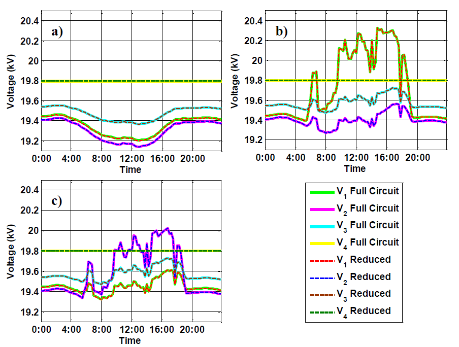
The same three simulations of the base case without solar, 1 MW PV at V₁, and 1 MW PV at V₂ are performed as time-series simulations for a 1-day period at 15 minute resolution. For the simulations, the load varies according to a standard load profile with the peak load in late afternoon. The peak load is shown in the “Initial 15-bus circuit simulation” figure, and all loads are varied together by a multiplier the rest of the day to match the feeder load profile. The impact on the voltages at the four buses-of-interest due to variations in the load is shown in the “Simulation of the full circuit and reduced circuit” figure. As seen in this figure, the reduced circuit has the same results as the full circuit even as the loads change throughout the day. The one-day simulations for a 1 MW PV plant connected at either V₁ or V₂ are shown in “Simulation of the full circuit and reduced circuit” figure’s part (b) and “Simulation of the full circuit and reduced circuit” figure’s part (c), respectively. The solar output profile for a cloudy day is simulated to show the impact of solar variability on the voltage and the corresponding time-series accuracy of the reduced model.

The reduced circuit is shown to be equal to the full feeder model for both snapshot simulations and time-series simulations with solar interconnected at two locations. The reduced circuit can accurately represent the time-varying nature of PV on the grid.

Conclusion

With an increasing amount of Distributed Generation (DG) being connected on the distribution system, a method for simplifying the complex system to an equivalent representation of the feeder is advantageous for streamlining the interconnection study process. The equations and methodology are presented for simplifying feeders to only specified buses-of-interest while maintaining accuracy and the feeder topology. Mathematical proofs were presented to show the equivalence of the reduced circuit for voltage drop, line losses, and circuit current power flow. The method is demonstrated on a 15-bus feeder with two buses-of-interest that is reduced to a 4-bus circuit. The steps of reduction are shown as an example with all calculated circuit parameters. The reduced circuit is validated with PowerWorld Simulator to have the same voltages and characteristics at the buses-of-interest as the original circuit.

The equivalent circuit reduction method accurately represents the full circuit for time-series simulations. Even with a time-varying load profile and variable solar generation, simulation of the reduced circuit performs the same and has equivalent voltages when validated against the full circuit. It was not demonstrated in simulation in this report, but the reduced circuit is also valid for simulating operations of voltage regulation equipment in the feeder because the voltage profile at any bus-of-interest was shown to be equivalent to the full circuit. Since the line current was also shown to be equal in the reduced circuit, the reduced circuit can also handle any voltage regulation equipment that contains a load drop compensator (LDC).

It is important to recall the assumptions necessary for the circuit reduction method. The assumptions about balanced phase current and neglecting shunt terms can be especially problematic for simulating distribution systems. In future work this method will be expanded to be able to handle more realistic distribution systems with full complexity. After validating the circuit reduction methodology, the method can be applied to feeders with different topologies to produce a better understanding of how many buses are required in the simplified model and to quantify the decrease in simulation times and other benefits.

References

- ↑ Sandia, Formulating a Simplified Equivalent Representation of Distribution Circuits for PV Impact Studies, April 2013, [Online]. Available: http://energy.sandia.gov/wp/wp-content/gallery/uploads/2013_SAND-CircuitReduction.pdf [Accessed April 2014].
- ↑ R. J. Broderick, J. E. Quiroz, M. J. Reno, A. Ellis, J. Smith, and R. Dugan, “Time Series Power Flow Analysis for Distribution Connected PV Generation,” Sandia National Laboratories SAND2013-0537, 2013
- ↑ J. E. Quiroz and C. P. Cameron, “Technical Analysis of Prospective Photovoltaic Systems in Utah,” Sandia National Laboratories SAND2012-1366, 2012
- ↑ M. J. Reno, A. Ellis, J. Quiroz, and S. Grijalva, “Modeling Distribution System Impacts of Solar Variability and Interconnection Location,” in World Renewable Energy Forum, Denver, CO, 2012
- ↑ J. Quiroz and M. J. Reno, “Detailed Grid Integration Analysis of Distributed PV,” in IEEE Photovoltaic Specialists Conference, Austin, TX, 2012
- ↑ 6.0 6.1 “WECC Guide for Representation of Photovoltaic Systems In Large-Scale Load Flow Simulations,” WECC Renewable Energy Modeling Task Force, 2010
- ↑ 7.0 7.1 7.2 7.3 W. H. Kersting, Distribution System Modeling and Analysis, Third ed. Boca Raton, FL: CRC Press, 2012
- ↑ L. Kijun and P. Song-Bai, “Reduced modified nodal approach to circuit analysis,” IEEE Transactions on Circuits and Systems, vol. 32, pp. 1056-1060, 1985
- ↑ T. H. Chen and S. W. Wang, “Simplified bidirectional-feeder models for distribution-system calculations,” IEE Proceedings – Generation, Transmission and Distribution, vol. 142, pp. 459-467, 1995
- ↑ T. Shimada, S. Agematsu, T. Shoji, T. Funabashi, H. Otoguro, and A. Ametani, “Combining power system load models at a busbar,” in IEEE Power Engineering Society Summer Meeting, 2000, pp. 383-388 vol. 1
- ↑ A. P. Thant, “Steady State Network Equivalents for Large Electrical Power System,” Masters Thesis, Electrical Engineering, Polytechnic University, 2008
- ↑ N. Vempati, R. R. Shoults, M. S. Chen, and L. Schwobel, “Simplified Feeder Modeling for Loadflow Calculations,” IEEE Transactions on Power Systems, vol. 2, pp. 168-174, 1987
- ↑ J. B. Ward, “Equivalent Circuits for Power-Flow Studies,” Transactions of the American Institute of Electrical Engineers, vol. 68, pp. 373-382, 1949
- ↑ “WECC Wind Power Plant Power Flow Modeling Guide,” WECC Wind Generator Modeling Group, 2008
- ↑ J. Brochu, C. Larose, and R. Gagnon, “Generic Equivalent Collector System Parameters for Large Wind Power Plants,” IEEE Transactions on Energy Conversion, vol. 26, pp. 542-549, 2011
- ↑ A. Ellis, M. Behnke, and C. Barker, “PV system modeling for grid planning studies,” in 37th IEEE Photovoltaic Specialists Conference, 2011, pp. 002589-002593
- ↑ 17.0 17.1 17.2 E. Muljadi, C. P. Butterfield, A. Ellis, J. Mechenbier, J. Hochheimer, R. Young, N. Miller, R. Delmerico, R. Zavadil, and J. C. Smith, “Equivalencing the collector system of a large wind power plant,” in IEEE Power Engineering Society General Meeting, 2006, p. 9 pp
- ↑ E. Muljadi, S. Pasupulati, A. Ellis, and D. Kosterov, “Method of equivalencing for a large wind power plant with multiple turbine representation,” in IEEE Power and Energy Society General Meeting, 2008, pp. 1-9
- ↑ J. Brochu, C. Larose, and R. Gagnon, “Validation of Single- and Multiple-Machine Equivalents for Modeling Wind Power Plants,” IEEE Transactions on Energy Conversion, vol. 26, pp. 532-541, 2011
- ↑ G. A. Mendonça, H. A. Pereira, and S. R. Silva, “Wind Farm and System Modelling Evaluation in Harmonic Propagation Studies,” in International Conference on Renewable Energies and Power Quality, Santiago de Compostela, Spain, 2012
- ↑ M. A. Elizondo, L. Shuai, Z. Ning, and N. Samaan, “Model reduction, validation, and calibration of wind power plants for dynamic studies,” in IEEE Power and Energy Society General Meeting, 2011, pp. 1-8
- ↑ 22.0 22.1 22.2 “Distribution Green Circuits Collaboration,” EPRI, Technical Report 1020740, 2010