
Author: National Renewable Energy Laboratory[1]
In this project, the National Renewable Energy Laboratory (NREL) developed a dynamic modeling process of the modules to be used as building blocks to develop simulation models of single PV arrays, expanded to include Maximum Power Point Tracker (MPPT), expanded to include PV inverter, or expanded to cover an entire PVP. The focus of investigation and complexity of the simulation determines the components that must be included in the simulation.
PV inverter manufacturers may be interested in the detail of PV inverter models with various control variables available. PV plant developers may be interested in the dynamic behavior of PVPs under transient events and the role of future PVPs to provide auxiliary services to the electric grid. Utility planners may be interested in investigating parallel operation with other renewable energy power plants, fault ride-through capability, and frequency response of the PVP.
Many PV installations are roof-top installations within the distribution power system, and are mostly funded by private homeowners or businesses. The advantages of this type of installation are ease of installation, diversity of solar irradiation (lower impact on voltage and frequency fluctuations), and no requirement for building new transmission lines.
Other PV installations are megawatt-scale PVPs located in remote, inexpensive locations within solar-rich regions. The use of transmission lines may be necessary to transmit the bulk power generated by these PVPs.
This report is arranged as follows: In Section 2, the basic PV module and PV array are presented. In Section 3, the PV inverter and detail controls are described. Many of the control functions are developed to comply with rules and regulations for installations at different locations. As the size of PV installations grow, the impact on distribution networks, and eventually on transmission networks, can be significant. PV manufacturers are striving to comply with local rules to expand their market share. Because many of the PV inverters are installed on the distribution network, symmetrical and unsymmetrical faults are covered in this section. In Section 4, PV inverter validation is presented based on field tests conducted at Southern California Edison. The validation includes both symmetrical and unsymmetrical faults. These testing efforts are important to validate the grid interface capability of PV inverters from different manufacturers. In Section 5, the conclusion of this report is presented.
Contents
- 1 Basic PV Module and PV Array
- 2 PV Inverter
- 3 PV Inverter Model Validation
- 4 Conclusion
- 5 References
Basic PV Module and PV Array
_and_model_results_(solid_line).png)
.png)
.png)
.png)
.png)
To understand the basic PV module and PV array characteristics, we use the I-V characteristics commonly found in manufacturing data sheets. PV module manufacturers use different solar cells; thus, it is expected that PV module characteristics are different from one manufacturer to another. Different qualities of solar cells are used by the same manufacturer for modules in market segments within the industry. In this section, current-voltage relationships of a single solar cell are expanded to a PV module and, finally, an array. There are numerous models for solar cell operation, but the five-parameter model is commonly adopted as it uses the current-voltage relationship for a single solar cell and only includes cells or modules in series.
Basic Solar Cell Characteristics
The characteristic of a solar cell is affected by solar irradiance and temperature. A PV module consists of multiple solar cells connected in series and parallel to achieve the desired voltage and current. An array of modules is usually interconnected in series and parallel in a direct current (DC) network; the output is optimized by MPPT. Although the characteristic of the PV module is usually provided by the manufacturer, the interconnected modules are used to form an array of PV modules to reach the specified voltage and current compatible with the power inverter.
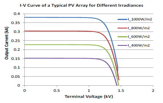
One or several MPPT are connected in parallel and then connected to a PV inverter to convert to the alternating current (AC) network. After voltage is stepped up by transformers, the output power is transmitted to the load center by an AC transmission line. A typical PVP may reach tens or hundreds of megawatts. When the output of the module is short-circuited, the short-circuit current (ISC) is limited at a certain value. This short-circuit value depends on the solar irradiance. When the output of the module is open-circuited, the voltage at open circuit is known as VOC.
The power characteristic of a PV module can be derived from the I-V characteristics. The power increases until it reaches optimal voltage (VOPT) at the knee point of the curve. Above the VOPT, PV output decreases until it reaches zero at open-circuit voltage. Below VOPT, PV behavior is similar to a current source, and above VOPT, PV behavior is similar to a voltage source. Presently, a PV inverter may have megawatt rating, and the trend seems to be toward larger sizes to accommodate large PVPs.
Other PV modules may behave differently, especially if the parameters of the solar cell deviate significantly from the one we used in this study. The steep slope is an important characteristic to have because solar irradiance changes by solar direction, cloud covering, and dust condition, and the changes in solar irradiance can occur very quickly. A decrease in solar irradiance at the same temperature in general shrinks the PV curve down.
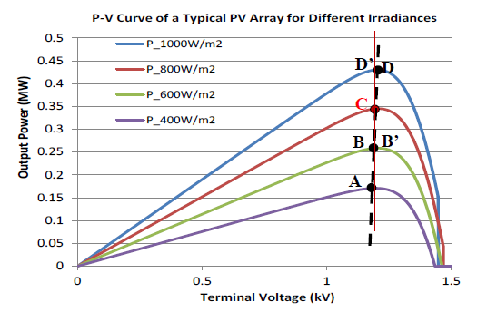
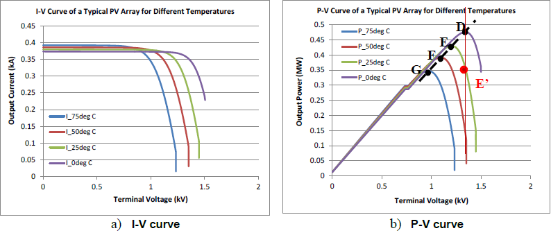
The optimum voltage moves to the lower values (path DEFG) as the temperature increases from 0°C (point D) to 75°C (point G). It is expected that solar irradiance will change more rapidly than temperature. Comparing the slopes of maximum line path as shown by line ABCD and DEFG the PV module range of voltage variation is more sensitive to temperature changes than solar irradiance changes. The same scenario as the changes in solar irradiance is applied to changes in temperature. Suppose that, originally, the operating point is at Point D, where the temperature is 0⁰C. As the temperature rises to 25⁰C, without MPPT, the operating point moves from Point D to Point E’, where, if we have an MPPT, the operating point could have been at Point E. The difference between output power production of Point E and power production at Point E’ is significant (PE >> PE’). This difference shows a significant power production loss. Fortunately, although the slope of line DEFG is low, the change in temperature does not occur as fast as the change of solar irradiance. The MPPT should have plenty of time to adjust to the new operating point.
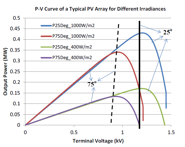
As solar irradiance and temperature change, the P-V curves shift down and to the left. This information is used to choose the voltage operating range, PV module output power, and PV inverter operating range. As shown Table below, the slope for 25⁰C is steeper than the slope for 75⁰C.
| Optimum Voltage With Corresponding Peak Power | ||
|---|---|---|
| At the DC Bus of the PV Inverter | Vpeak (kV) | Peak Power (MW) |
| 25°C at 1000 W/m^2 | 1.204588 | 0.430284 |
| 75°C at 1000 W/m^2 | 0.951484 | 0.340844 |
| 25°C at 400 W/m^2 | 1.19622 | 0.171 |
| 75°C at 400 W/m^2 | 0.932 | 0.133874 |
| Slope for 25°C = 30.98518 MW/kV | ||
| Slope for 75°C = 10.62256 MW/kV | ||
Equivalent Circuit of a Solar Cell and PV Module
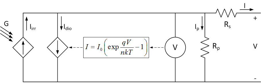
The equation governing the internal currents of a solar cell can be expressed based on Kirchhoff Current Law as
\(I = I_{irr} – I_{dio} – I_{p}\)where:
- Iirr is the photo current or irradiance current, which is generated when the cell is exposed to sunlight
- Idio is the current flowing through the anti–parallel diode, which induces the nonlinear characteristics of the solar cell
- Ip is the shunt current due to the shunt resistor RP branch
Substituting relevant expressions for Idio and Ip, we get
\(I = I_{irr} – I_{0} \left[exp \left(\frac{q(V+IR_{s})}{nkT} \right)-1 \right]-\frac{V+IR_{s}}{R_{p}}\)where:
- q is the electronic charge (q = 1.602 × 10⁻¹⁹ C)
- k is the Boltzmann constant (k = 1.3806503 × 10⁻²³ J/K)
- n is the ideality factor or the ideal constant of the diode
- T is the temperature of the cell
- I0 is the diode saturation current or cell reverse saturation current
- RS and RP represent the series and shunt resistance, respectively
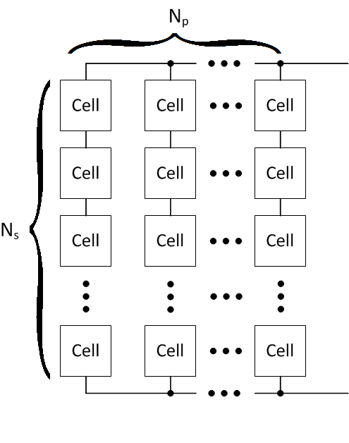
Because a solar cell is generally rated at low voltage and low current, commercial PV manufacturers connect the solar cells in series and parallel to form a PV array, module, or panel. A PV array is typically composed of solar cells in series and strings in parallel. It is important to consider the effects of those connections on performance. The output current IA and output voltage VA of a PV array with NS cells in series and NP strings in parallel is found from the following equation
\(I_{A} = N_{p}I_{irr} – N_{p}I_{0} \left[exp \left(\frac{q \left(V_{A}+I_{A}\frac{N_{S}}{N_{P}}R_{S} \right)}{N_{S}nkT} \right)-1 \right]-\frac{V_{A}+I_{A}\frac{N_{S}}{N_{P}}R_{S}}{\frac{N_{S}}{N_{P}}R_{P}}\)The values for Irr and Io must be compensated for different temperatures and solar irradiance.
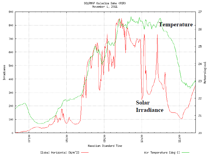
\(I_{irr} = I_{irr,ref} \left(\frac{G}{G_{ref}} \right)\cdot1+\alpha’_{T}(T-T_{ref})\) \(I_{0} = I_{0,ref} \left[\frac{T}{T_{ref}} \right]^3\cdot\exp \left[\frac{E_{g,ref}}{kT_{ref}}-\frac{E_{g}}{kT} \right]\)In addition, the values of Rs, Rp, Irr,ref, and Io,ref can be found from the data specification or from the experiment. Using the equation above, one can derive the parameters using experimental data with the corresponding adjustment for solar irradiance and temperature. The variation of solar irradiance from zero to peak can be very fast because of passing clouds. For example, the variation of solar irradiance between 10 a.m. and 10:30 a.m. is large and active. However, keep in mind that the measurement is taken at a single spot. For large PV plants covering a very large area, there will likely be some smoothing effect; thus, the impact on the power system may not be as bad as a single-spot solar irradiance measurement. The temperature variation over the 12-hour period for this particular day is narrow (less than 7º within 12 hours). The step changes in temperature are not as steep as the solar irradiance variations. Note that the temperature T and Tref in the equations presented above are based on the unit of Kelvin, and it is the junction temperature of the solar cell; however, because the surface of the solar cell is very large, the changes and the rate of change in the solar cell will not be substantially different from air temperature.
A series of validation tests comparing actual versus analytically predicted results was conducted at the University of Colorado at Denver, and it was observed that the equations for Iirr can predict the actual I-V characteristic of the PV module. It also shows the impact of series connection and solar irradiance on the instantaneous I-V curves. The characteristic of a solar cell is affected by solar irradiance and temperature of the module. A PV module consists of multiple solar cells connected in series and parallel to achieve the desired voltage and current. An array of modules is usually interconnected in series and parallel in a DC network, and the output is optimized by MPPT. While the characteristic of the PV module is usually provided by the manufacturer, the interconnected modules are used.
Maximum Power Point Tracking
To maximize output power, an MPPT is commonly used to track the maximum power point (MPP). In principle, as shown in the previous section, the terminal voltage can be used to vary the output power. For example, if operating at a voltage below the optimal point, by increasing the terminal voltage at constant solar irradiance, the output current of the PV module is constant, and the output power of the PV module and PV array thus increases until the maximum point is reached. If we continue to increase the terminal voltage beyond that point, the DC output current decreases as a faster rate, and output power decreases.
Thus, in this topology the key to maximizing the output power of a PV array or PV module is to control the terminal voltage of the PV array. In this section, we describe several methods used to track the MPP. Modifications will be necessary to achieve MPP tracking for large multi-stage or more complex multi-level inverters.
The solar cell is connected as a PV array with series and parallel interconnection and is connected to an MPPT. The MPPT is represented as an adjustable DC-dependent voltage source. In the following section, several methods of MPPT are described.
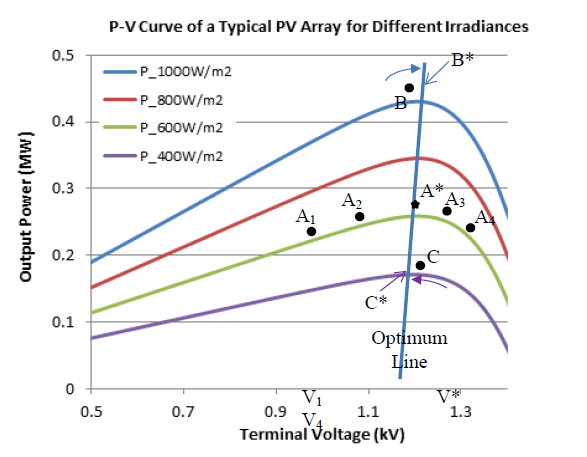
To illustrate MPPT, let’s use Figure on the right. The P-V curves are shown for different solar irradiances. The optimum operating voltage can be approximated by the thin blue line labeled “Optimum Line.” This is the line where the MPP will operate as the solar irradiance changes. Assume the solar irradiance is at 600 W/m^2 (the green curve). In the beginning, the operating point is at Point A1 at the voltage V1. As the voltage is raised from V1 to V4, the operating point moves from Point A1to A2 and eventually reaches the maximum point at A* at V*. As the voltage is increased, the operating point reaches Point A3 and eventually will reach Point A4 at voltage V4. Thus, it shows that to modify the operating point, we can change the terminal voltage of the PV module, and there will be only one maximum operating Point A* for a particular solar irradiance and temperature. For all practical purposes, the temperature is assumed to be constant compared to the changes in solar irradiance. The detection of maximum power and the direction of the voltage change are described in the next few sections.
Assume that we are operating at Point A*, and suddenly the output power drops. We know that the drop in power is caused by the reduction in solar irradiance. Here, as an example, the output power was originally PA*, with operating point A*. A sudden drop of power from PA* to PC at constant, the terminal voltage V* indicates that the solar irradiance decreases. In this case, it drops from 600 W/m^2 to 400 W/m^2. Following the path of the optimum line, the terminal voltage must be reduced from VC to VC* to get to Point C* as indicated by the purple arrow, and the new output power will be PC*.
The same can be said for a condition in which the solar irradiance increases from 600 W/m^2 to 1000 W/m^2 at constant voltage V* (operating point moves from Point A* to Point B). Based on the optimum line path, terminal voltage must be raised from voltage V* to voltage VB*, as indicated by the blue arrow.
Hill Climbing Method
This method is the most basic of MPPT. In this concept, the output of the PV array is adjusted by controlling the output terminal voltage of the PV array VA. By varying the output voltage VA, the output power of the PV array will vary as well. At the optimum voltage (VOPT), the output power is maximized. This technique is specific to this inverter type and will have to be modified for use with different inverter topologies.
To simplify, assume that the VA is varied as a triangular fashion about VOPT. As the output voltage VA is varied from the low (VLO) to the upper limit (VHI) and then back to VLO, the output power varies in the same fashion. Below VOPT, the PV array behaves likes a current source, and above the VOPT, it behaves like a voltage source. At the transition from the current source behavior to the voltage source behavior, the optimum point is located.
Figure on the right shows the terminal voltage variation used to search for the MPPT. The range of voltage used between VHI and VLO is determined by the optimum line slope and solar insolation range. Also, some overhead must be included to allow for temperature variation during the four seasons of the year. Note that the voltage range can be adjusted to make the search more efficient by compensating for the operating temperature.
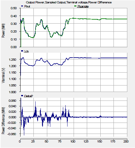
As the VA varies, the corresponding output power also varies. Note that the waveform has a rounded corner indicating nonlinearity in the region close to the optimum or peak power. Using a sample-and-hold (“sampler”), we digitized the output power signal and labeled it Psample.
The difference between the output power, Pout, and the Psample, DeltaP, is shown in figure on the right. Because the sampling rate is constant, the power difference DeltaP can be considered the derivative of the output power and can be used to lead direction of the maximum output power.
DeltaP varies with time. Note that DeltaP changes the sign as it crosses the MPP. As the output voltage VA is varied from low to high and back to low, the output power varies in the same fashion. Below VOPT, the PV array behaves like a current source, and above the VOPT, it behaves like a voltage source. As explained before, the DeltaP is an indication of the direction that the terminal voltage must be adjusted. The positive DeltaP indicates that the optimum point has not been reached and the terminal voltage must be increased. Similarly, the negative DeltaP indicates that the optimum point has not been reached and the terminal voltage must be decreased.
At the transition from the current source behavior to the voltage source behavior, the optimum point is located. This transition can be detected by a comparator, and the output of the comparator can be used to signal that the optimum point has been reached and the searching effort can be stopped until a new condition is detected (e.g., the change in solar irradiance).
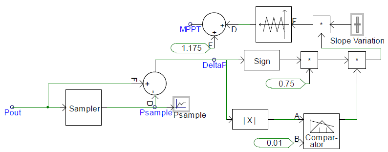
The triangular wave is used to search the MPP. The triangular waveform has two parameters, VHI and VLO, and an input F to adjust the frequency (slope) of the triangular waveform. The frequency of the triangular waveform is set by the constant value, which can be set by the slider (“Slope Variation”). Initially, the frequency of the triangular waveform is kept constant to generate a 10-Hz triangular waveform. Once the MPP is found, the search must be stopped, and the PV inverter will operate at this MPP, generating a constant terminal voltage VA=VOPTIMUM.
The DeltaP is used to indicate that the operating point is non-optimum, and MPPT continues to search. The comparator will detect the non-optimum operation and will output Logic 1. When the optimum operation is reached, the logic turns to zero. The comparator is used to detect the positive DeltaP and the negative DeltaP. Once the optimum terminal voltage VA=VOPTIMUM is reached, the input F is set to 0, and the output MPPT is fixed at VOPTIMUM. The sign function is used to change the direction of the search. When DeltaP is positive, MPPT will increase the terminal voltage VA, and when the DeltaP is negative, MPPT will decrease the terminal voltage VA. The gain 0.75 should be tuned to get the best response. Potentially, this gain can be used to adjust the gain based on temperature.
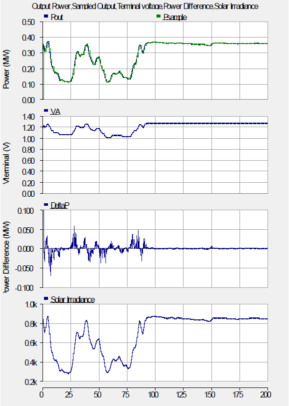
Figure on the right shows a subset (a small time slice) of recorded solar irradiance data measured at the airport in Honolulu, Hawaii. A segment of time within 200 seconds was chosen to show the dynamic of the solar irradiance. The data sampled at 1 Hz shows the variation of the level of solar irradiance. The output power of the PV array follows the variation of the solar irradiance. The corresponding terminal voltage (voltage VA) tracks the maximum point very closely and is also shown to react to the changes in solar irradiance. Note that the variation of the terminal voltage is limited between 1.0 kV and 1.35 kV to follow the available I-V curve used in this study. This is accomplished by setting the triangular waveform VHI = 0.175 kV and VLO = -0.175 kV and an offset of 1.175 kV. The terminal voltage will range from 1.0 kV to 1.35 kV. This voltage range is dependent on the temperature of the solar cell and must be adjusted accordingly. As mentioned in the previous sections, the temperature change occurs very slowly compared with the changes in solar irradiance.
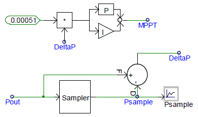
Zero Steady-State Error DeltaP
This method is very basic in that the DeltaP is sampled at a constant rate, and its value can be considered the true derivative of the output power. Similarly, the PI controller will yield a zero steady-state error. By using a simple PI controller, we can drive the DeltaP to zero. The outcome of this controller seems to follow the same trend as the Hill Climbing Method, with the PI controller indicating a slightly smaller average value of DeltaP, although with a proper tuning, the difference can be insignificant.
In this method, no triangular waveform is used. However, the PI controller has two parameters (VHI and VLO) that must be set to limit the voltage. When the output reaches higher than VHI, the integrator freezes, and output is held at VHI. Similarly, when PI controller output reaches below VLO, the integrator freezes. Another parameter used is the proportional and integral gain of the PI controller.
MPPT tracks the solar irradiance very closely as driven by the PI controller to reach 0 dP/dV. The DeltaP shows a large deviation at the beginning of the simulation. However, toward the end of the simulation, the error DeltaP gets smaller, indicating that the PI controller tracking performance improves as time progresses.
MPPT by Detection of Power Pulsations
This method is very similar to zero steady-state error. In this concept, terminal voltage is also modulated by using the triangular waveform (0.5 Hz); however, another small triangular signal at higher frequency (10 Hz) is added to the top of the main triangular waveform.
Figure on the right shows the double triangular waveforms used to modulate the terminal voltage. The slower variation of the triangular waveform is intended only to vary the terminal voltage VA, while the smaller triangle at high frequency signal is used to probe the proximity of the operating point to the MPP at any condition. Once this MPP condition (shown by the red ellipse solid line in b) is reached, the search must be stopped, and the terminal voltage should be kept constant until the solar irradiance changes and the frequency doubling disappears. If the output power Pout is passed through the band-pass filter with the center frequency equal to the small triangle signal, the output of the band-pass filter is minimized when the MPP is reached, indicating that the frequency doubling has also been reached (shown by the dashed red ellipse line in b).
When the terminal voltage varies to follow the triangular waveform, the output power increases until the optimum operating point is reached. At this peak power, the output power will contain the twice the frequency of the small signal triangular waveform. For example, if the triangular waveform has a frequency of 5 Hz at the output power, the output power will have the 10-Hz component. Thus, the output of the band-pass filter is minimized.
Another possible indicator to signal the MPP is to use the output power pulsation. It is shown that the output power pulsation is minimized and the optimum frequency has been reached.
PV Inverter
![]()
![]()
![]()

_-_(a)_three-phase_equivalent_circuit_and_(b)_positive-sequence_equivalent_circuit.png)
_(a)_three-phase_voltage_and_(b)_three-phase_inverter_output_currents.png)
_grid_contribution_and_(b)_PV_inverter_contribution.png)
_three-phase_voltage_and_(b)_three-phase_inverter_output_currents.png)
_grid_contribution_and_(b)_PV_inverter_contribution.png)
_grid_voltage,_(b)_three-phase_inverter_output_currents,_and_(c)_grid_currents.png)
_grid_voltage,_(b)_three-phase_inverter_output_currents,_and_(c)_grid_currents.png)
![]()
![]()
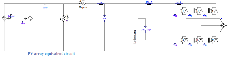
The PV inverter is the point of conversion from DC to AC power. In small residential applications, the PV inverter is usually single-phase, converting DC to single-phase AC (60 Hz). The PV array is connected to the PV inverter via MPPT to optimize energy conversion from sunlight to electrical power. A detailed discussion is not included in this report. The PV inverter for large-scale installation usually comes in three-phase arrangements. The PV inverter combines the output of rows of PV strings in DC and converts them to AC. For example, the inverter can processes the output of a PV array with 500 PV modules. Three-phase output rated at 208 V or 480 V is commonly found in commercial PV inverters. It must be emphasized once again that the topology described here is a single stage topology and controls for multi-level and multi-stage converters will require significant modifications from the ones described here.
The PV inverter consists of three pairs of power electronics switches (commonly implemented with an insulated gate bipolar transistor, or IGBT). As shown in Figure on the right, the top switches connect the terminals of Phase A, Phase B, or Phase C to the positive bus, and the bottom switches connect the phases to the negative bus of the DC bus. In each pair, the top and bottom switches are never turned on at the same time to avoid shorting the DC bus. The switching pattern and topology vary depending on the application. In most applications, the three-phase inverters are controlled as a current-regulated pulse width modulation (PWM). These modulation techniques have evolved from simple to more complex techniques, especially in the drives applications. For each top IGBT, there is a corresponding diode (also called a free-wheeling diode) to allow reverse current direction from terminal to the positive bus of the DC bus. Similarly, each bottom IGBT has a free-wheeling diode to let the current flow from the negative bus to the terminal.
Dynamic Modeling of PV Inverter
The dynamic modeling of a PV inverter from the grid perspective is similar to the grid-side inverter found in a Type 4 wind turbine generator, also known as a full converter wind turbine. It effectively decouples the PV from the grid, improving fault response in both. Electrical transient faults occurring in the transmission lines are buffered by the PV inverter to prevent damage to the PV panels. Similarly, the transients on the DC side created by the PV generation because of passing clouds are buffered from directly affecting the power grid on the AC side. It allows the PV panels to operate over a wide operating range, leading to improved power extraction from the solar irradiance. The converter interfacing the PV array to the grid has to process the entire output of the PV array. This report specifically deals with these larger inverters. Future work will be done on multi-stage inverters which have some additional flexibility.
Control of PV Inverter
AC Current Control
The PV inverter is a mature technology developed early on by the power drives industry for adjustable-speed drives, also known as adjustable-frequency drives, used to control variable-speed operation of electric machines (e.g., induction motors) with torque or speed-control capability. Thus, the basic operations have been developed based on the experience gained by the electric drives industry. The application of these technologies to PV requires modifications since there are no motors present.
The ability to control the current output of the power converter both in magnitude and phase angle enables the power inverter to precisely control the fluxes of the electric motors, thus allowing the precise control of torque or speed using the technique known as “flux control” or “vector control.” The capabilities to control output current are applicable to PV inverter applications, with the capability to limit the over current during short circuit and adjust the power factor or reactive power or voltage very precisely.
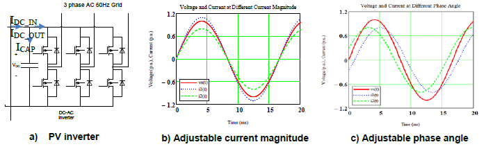
The PV inverter shown in Figure on the right (a) is a current-controlled, voltage-source inverter. It can generate current that varies in its magnitude and phase angle. In (b), the output current is precisely controlled to be 0.8 p.u. and 1.1 p.u. Similarly, the phase angle can be controlled with respect to the voltage. For example, in (c), the phase angles of the output current are controlled to be leading and lagging the voltage by 20 degrees. Although changing the magnitude of the current in phase with the voltage will change the real power output only, changing the phase angle of the current will change both the real and reactive power output of the inverter.
The DC-AC conversion is accomplished using a current-controlled inverter, which controls the real and reactive output power. Although the focus in this report is on the specific topology mentioned, various converter topologies can be modeled with simple modifications using the same framework.
Real and Reactive Power Control of PV Inverter
Current control is used to control the output current (IPV). The output current components (IRE and IIM) can be controlled independently, where IRE is aligned with the voltage VS and IIM in quadrature with the voltage VS.
With current control capability of the PV inverter, real and reactive power output can be achieved independently and instantaneously.
\(P_{PV} = 3\cdot V_{PV}\cdot I_{Re}\) \(Q_{PV} = 3\cdot V_{PV}\cdot I_{Im}\)In this example, per-phase terminal voltage is VPV, and the line current IPV is the output current. Both voltage and current are the effective (RMS) values of the fundamental component (60 Hz). Usually, the voltage and current harmonics are small in modern power converters with high switching frequency. The output current must be passed through the weakest link (in terms of overcurrent rating) of the PV inverter (i.e., the power semiconductor IGBT switches). Power semiconductor switches for most commercial PV inverters are designed to carry 1.1 p.u.; however, the actual rating typically carries the peak (not RMS) of the overload current.
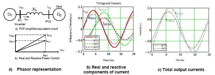
Figure on the right (a) represents a PV plant outputting power to the grid. The real and reactive components of the current (IRE and IIM) are represented in its phasor representation. In (b), the time domain is represented by the voltage vs(t), and the real iRE(t) and reactive iIM(t) current components are represented in time domain. The real power component of the current iRE(t) is in phase with the voltage source vs(t), while the reactive power component of the current iIM(t) is in quadrature with respect to the voltage source vs(t). In (c), the total output currents representing the same real power output adjusted at two different reactive power are represented as ipv1(t) and ipv2(t).
From (a) and (c), we can see that the output current ipv2(t) has a larger magnitude than the current ipv1(t); however, it is from (a) that the size of the real and reactive power output can be clearly identified by the phasors IRE1, IIM1, and IIM2, where the subscript RE indicates the current component in phase with the terminal voltage and the subscript IM indicates the current component quadrature with the terminal voltage.
Current-Regulated Voltage Source Inverter
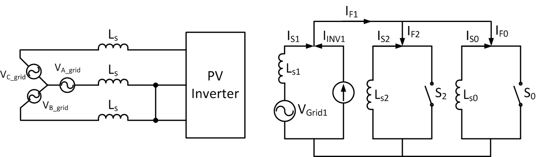
To describe the operation of the PV inverter, the equivalent circuit of the PV inverter connected to the grid is redrawn in Figure on the right. The PV inverter uses the voltage Vgrid to synchronize the power converter to the grid by using the phase-locked loop (PLL) to track the phase angle of the grid voltage. Thus, any changes in the phase angle or frequency will be followed as the power converter is locked to the grid voltage.
The three-phase voltage and line currents in time domain is then converted into dq axis in synchronous reference frame via Clarke Transformation and Park Transformation. In this section, only the voltage transformation is shown. The same transformation is also used for the currents. The three-phase quantities of the voltage in time domain can be written as
\(v_{a}(t) = V_{m}\cdot cos(\omega t)\) \(v_{b}(t) = V_{m}\cdot cos(\omega t – 120°)\) \(v_{c}(t) = V_{m}\cdot cos(\omega t + 120°)\)The Clarke Transformation changes the three-phase a,b,c stationary reference frame into the coordinate 𝛼,𝛽,0 in the stationary reference frame. The Clarke Transformation can be written as follows
\(\begin{bmatrix}V_{\alpha}\\
V_{\beta}\\
V_{0}
\end{bmatrix} =
\frac{2}{3}
\begin{bmatrix}
1 & -0.5 & -0.5\\
0 & 0.866 & -0.866\\
0.5 & 0.5 & 0.5
\end{bmatrix}
\begin{bmatrix}
V_{a}\\
V_{b}\\
V_{c}
\end{bmatrix}\)
The Park Transformation changes the variables in 𝛼𝛽0 axis (in stationary reference) into variables in dq0 axis (in synchronous reference frame). The Park Transformation can be written as follows
\(\begin{bmatrix}V_{d}\\
V_{q}\\
V_{0}
\end{bmatrix} =
\begin{bmatrix}
cos(\theta) & sin(\theta) & 0\\
-sin(\theta) & cos(\theta) & 0\\
0 & 0 & 1
\end{bmatrix}
\begin{bmatrix}
V_{\alpha}\\
V_{\beta}\\
V_{0}
\end{bmatrix}\)
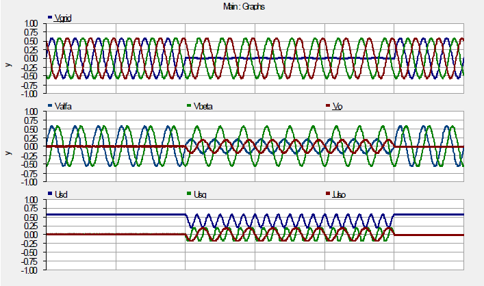
The Clarke and Park transformations transform the three-phase a,b,c in stationary reference frame into coordinate d,q,0 in synchronous reference frame. The three-phase grid voltages (va, vb, vc) are converted to voltage in 𝛼𝛽0 axis and finally into the dq0 axis (vd, vq, v0). The v0 component does not exist in a balanced symmetrical condition. The Clark and Park transformations transform the voltage a,b,c in time domain into voltage d,q,0 in the synchronous reference frame expressed as Usd, Usq, and Us0. The synchronous reference frame is aligned to Phase A of the three-phase Vgrid. The d-axis voltage Usdis maximum, and the q-axis voltage Usq ~ 0. For the voltages at the other nodes of the power system network, if there is a significant phase angle difference from the Vgrid, the representation of the voltages in dq0 axis will be different, and the Usq may not be equal to zero.
The Clark and Park transformations transform the voltage a,b,c in time domain into the voltage d,q,0 in the synchronous reference frame expressed as Usd, Usq, and Us0. The synchronous reference frame is aligned to Phase A of the three-phase Vgrid. The d-axis voltage Usd is maximum, and the q-axis voltage Usq ~ 0. For the voltages at the other nodes of the power system network, if there is a significant phase angle difference from the Vgrid, the representation of the voltages in dq0 axis will be different and the Usq may not be equal to zero. The intermediate values of the voltage output of the Clarke transformation changes the three-phase a,b,c stationary reference frame into coordinate α,β,0 in stationary reference frame. Note that the phase-angle shift in the a,b,c voltages is 120° with respect to one another, while in the 𝛼,𝛽,0 it is 90° with respect to one another. The zero sequence only presents in the unbalanced faults involving the ground with the certain connections of the transformers.
During a single-line-to-ground fault (phase A), Phase A voltage is grounded, and the flat line of Phase A voltage indicates a faulted phase. Representation in the dq0 axis is slightly different. During an SLG fault, the Usq and Usd have oscillating components at 120 Hz, indicating the presence of the negative-sequence voltage. The zero-sequence voltage Us0, however, shows a small 60-Hz oscillation.
The Inverse Clarke Transformation changes the variables in 𝛼𝛽0 axis (in stationary reference frame) into abc axis (in stationary reference frame). The Inverse Clarke Transformation can be written as
\( \begin{bmatrix}V_{a}\\
V_{b}\\
V_{c}
\end{bmatrix} =
\begin{bmatrix}
1 & 0 & 1\\
-0.5 & 0.866 & 1\\
-0.5 & -0.866 & 1
\end{bmatrix}
\begin{bmatrix}
V_{\alpha}\\
V_{\beta}\\
V_{0}
\end{bmatrix}\)
Similarly, the Inverse Park Transformation changes the variables in dq0 axis (in synchronous reference frame) into 𝛼𝛽0 axis (in stationary reference). The Inverse Park Transformation can be written as
\( \begin{bmatrix}V_{\alpha}\\
V_{\beta}\\
V_{0}
\end{bmatrix} =
\begin{bmatrix}
cos(\theta) & -sin(\theta) & 0\\
sin(\theta) & cos(\theta) & 0\\
0 & 0 & 1
\end{bmatrix}
\begin{bmatrix}
V_{d}\\
V_{q}\\
V_{0}
\end{bmatrix}\)
The real and reactive power can be computed as
\(P = \frac{3}{2}\cdot (V_{q}I_{q}+V_{d}I_{d})\) \(Q = \frac{3}{2}\cdot (V_{q}I_{d}-V_{d}I_{q})\)Given the references for real and reactive power, the reference currents can be found as
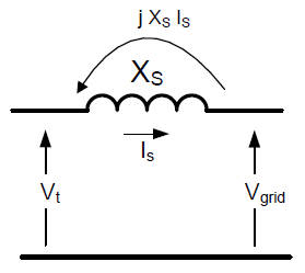
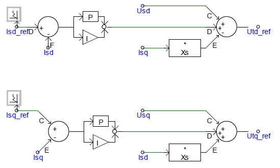
\(I_{dref} = \frac{\frac{2}{3}P_{ref}-V_{q}I_{q}}{V_{d}}\) \(I_{qref} = \frac{V_{q}I_{d}-\frac{2}{3}Q_{ref}}{V_{d}}\)In some cases, the reference voltage used is a remote bus from the terminal of the PV inverter. For example, the reference bus used is the Vgrid, and the impedance between the terminal and the Vgrid is given as impedance Xs. In this case, voltage drop across the impedance Xs is commonly compensated to get the required voltage that must be generated at the terminal of the PV inverter. Including the voltage drop across the Xs, the terminal voltage Vt can be computed as
\(V_{t} = V_{grid}+jX_{s}I_{s}\)It is implemented in the control diagram as
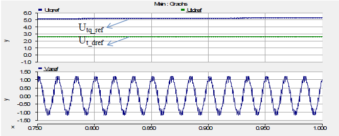
\(U_{tq}-jU_{td} = (U_{sq}-jU_{sd})+jX_{s}(I_{sq}-jI_{sd})\) \(U_{tq} = U_{sq}+I_{sd}X_{s}\) \(U_{td} = U_{sd}-X_{s}I_{sq}\)Or, given in the dq axis and including the current references, the voltage equations are implemented to get the voltage reference in the dq axis. The voltage references given in the dq axis are then converted back to the abc axis using the Inverse Park Transformation, and the voltage reference in the abc axis can be used to control the power inverter.
Figure below shows the voltage references presented in the dq axis and the Phase A voltage. The dq axis in synchronous reference frame, as shown, is almost flat lines, while the Phase A voltage is a sinusoidal wave form.
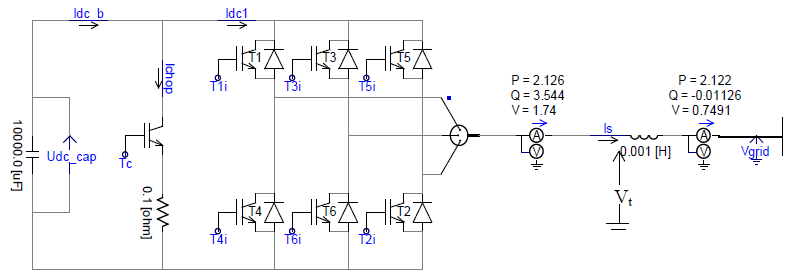
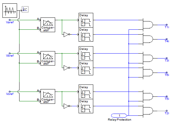
The voltage reference (in three-phase) is then compared with the triangular waveform at constant frequency, and the comparator output is split into two outputs. One is the logic signal used to turn the top switch in the power inverter on and off; the other is passed through the inverter logic to get the complement of the original signal. The complement signal is used to control the bottom switches of the power inverter. Note that the small time delay is introduced to avoid short-circuit of the DC bus so that the top and bottom switches do not turn on at the same time. Using the logic signals T1i, T2i, T3i, T4i, T5i, and T6i, the power switches are turned on and off to develop the desired output based on the real and reactive power commands. These logic signals can be disabled based on the protection scheme designed by the manufacturer. For example, a manufacturer may decide to turn off the power converter after a three-phase fault developed for 20 cycles and extend to 50 cycles for an SLG fault. Other manufacturers may have different schemes, and in many cases, it depends on the rules and regulations set by the host utilities that own the distribution network to which the PV inverter is connected.
Operation of the Inverter with MPPT
Many methods can be used to implement MPPT on the PV inverter. One way is to use a DC-DC converter between the PV array and the DC bus. In this way, one can keep the DC bus voltage while varying the PV array terminal voltage to find the MPPT function. Another method is to use a floating DC bus, as described in the following subsections.
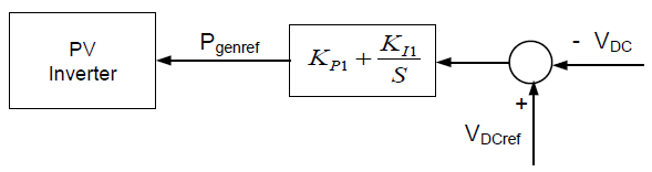
DC Bus Voltage Control
In the PV inverter, the output current is controlled to accomplish two main objectives: maximizing the output power and controlling the reactive power delivered to the grid. The power converter is usually controlled to have a constant DC bus. The DC bus voltage has a DC capacitor, where the average input current entering the DC capacitor must be zero. Maintaining the DC bus constant can be accomplished by ensuring that the real output power is controlled to balance the real power entering and leaving the DC bus. The voltage across the capacitor is the DC bus voltage. It can be written as
\(v_{DC} = \frac{1}{C}\int \left(i_{DC-IN}-i_{DC-OUT} \right)dt\)Maintaining the DC bus voltage constant means that the power entering the DC bus and the power leaving the DC bus is the same, thus the average charging current ICAP = 0. The balance between input and output power of the DC bus is maintained by controlling the DC bus constant. The DC bus voltage error is used to drive the output power of the PV inverter Pgenref for a system with a DC bus constant. For a system using a floating DC bus voltage as an MPPT, this reference can be used as an input to MPPT.
MPPT Implementation With DC Bus Voltage Control
In this aticle, we used a floating DC bus to maximize the output power. This method has been described in more detail in a paper[2]. In this way, the DC bus is directly connected to the PV array terminal output with the DC bus floating. Note that the operation of the PV inverter with this method is quite safe. For example, the PV array slope is relatively steep; thus, the difference in the DC bus voltage between optimum voltage (Vopt), where peak power value occurs, and open-circuit voltage is minimal. As shown in the I-V characteristic of a solar cell or PV array, the PV array produces less power as its terminal voltage exceeds its optimum voltage. This voltage self-limiting characteristic of the PV array is the reason we attempted to deploy this method.
As described here, the DC bus voltage depends on the simple balance equation of the power flow in the PV inverter. If the power input is larger than the power output, the voltage across the DC bus capacitor will increase. Similarly, if the power output is larger than the power input, the voltage across the capacitor will decrease. Or in terms of the DC currents we can express as (iDC-OUT < iDC-IN), then vDC increases and if (iDC-OUT > iDC-IN), then vDCdecreases. Thus, we use this characteristic to modulate the DC bus voltage. To avoid the controller malfunction, a dynamic braking can be implemented to detect an overvoltage condition, thus protecting the power semiconductor switches (IGBTs) from being exposed to excessively high DC bus voltage.
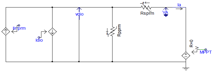
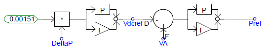
In Figure on the right, the control diagram to implement MPPT is modified. The signal output of the PI controller labeled MPPT is replaced by Vdcref in this control block diagram. This is the reference Vdc that should be used to control the DC bus voltage to reach MPPT. This value is compared with the actual DC bus voltage, labeled VA. The error is used to control the reference output power of the PV inverter. Based on the goal of maintaining the balance of power within the DC bus capacitor as described here, increasing output power faster than the increase in input power will reduce the DC bus voltage, and decreasing output power slower than the increase in input power will increase the DC bus voltage.
For example, the PV inverter current-regulated voltage source inverter (CR-VSI) is controlled by using MPPT with the PI controller described here. In Figure on the right, the output power is shown to follow the solar irradiance with the derivative of output power deltaP (dP/dt) used to drive the direction of the terminal voltage of the PV array (VA). Note that the range of the terminal voltage variation is not very large for the specific solar cell we used. This makes it easier to specify the voltage ratings of the PV inverter components without having to design with large headroom. The Figure below shows the output voltage and output current of the PV inverter with MPPT implemented. As shown from the graph, the voltage and the output current waveform are smooth, and the MPP tracking does not appear to influence the output voltage and currents.
Operation of the Inverter Under Fault Conditions
Symmetrical Component Theory
The method to analyze power systems under unbalanced conditions was developed by C.L. Fortesque in 1918. He developed the concept to explain the behavior of unbalanced conditions in steady-state analysis. He developed a theory that any unbalanced poly-phase phasor quantities can be analyzed using:
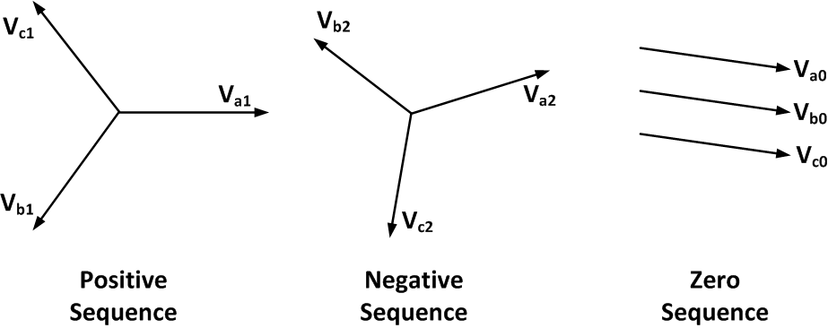
- A balanced set of phasors with a positive sequence (abc sequence)
- A balanced set of phasors with a negative sequence (acb sequence)
- A set of three equal phasors, also known as zero sequence.
Fortesque developed a transformation to decompose a multiphase unbalanced system of n related phasor quantities into n systems of balanced phasors called the symmetrical components of the original phasors. The transformation to convert from the three-phase unbalanced voltage phasors into the symmetrical components can be expressed as a three-by-three matrix expressed in complex numbers or in a polar form
\( \begin{bmatrix}V_{0}\\
V_{1}\\
V_{2}
\end{bmatrix} =
\frac{1}{3}
\begin{bmatrix}
1 & 1 & 1\\
1 & a & a^2\\
1 & a^2 & a
\end{bmatrix}
\begin{bmatrix}
V_{a}\\
V_{b}\\
V_{c}
\end{bmatrix}\)
where V0, V1, V2 are the symmetrical components of the voltage phasors representing Va0, Va1, Va2.
The subscript 0 represents the zero-sequence phasors, the subscript 1 represents the positive-sequence phasors, and the subscript 2 represents the negative-sequence phasors.
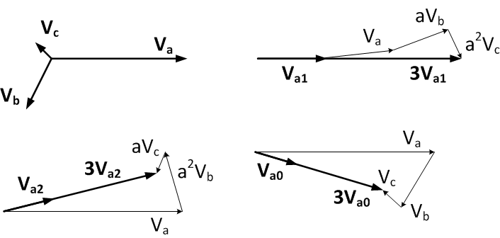
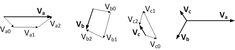
As an example, a unbalanced voltage can be decomposed into its symmetrical components. The symmetrical components Va0, Va1, Va2 can be found by applying the phase shifter variable “a.”
The quantity “\(a\)” can be expressed in complex notation or polar notation. Any phasor multiplied by “\(a\)” is rotated clockwise by 120°. Similarly, any phasor multiplied by “\(a^2\)” is rotated clockwise by 240°.
\(a = e^{j\frac{2\pi}{3}} = -\frac{1}{2}+j\frac{\sqrt3}{2}\) \(a^2 = e^{j\frac{4\pi}{3}} = -\frac{1}{2}-j\frac{\sqrt3}{2}\)The transformation to convert from the symmetrical components of the voltage phasors into the three-phase voltage phasors can be expressed as a three-by-three matrix
\( \begin{bmatrix}V_{a}\\
V_{b}\\
V_{c}
\end{bmatrix} =
\begin{bmatrix}
1 & 1 & 1\\
1 & a^2 & a\\
1 & a & a^2
\end{bmatrix}
\begin{bmatrix}
V_{0}\\
V_{1}\\
V_{2}
\end{bmatrix}\)
As an example, a three-phase unbalanced voltage can be reconstructed from its symmetrical components (positive, negative, and zero sequence).
Symmetrical Fault (3-LG)
The symmetrical fault occurs when all three phases are connected to the ground. These faults occur, for example, when a tree falls on the lines and creates a short circuit to the ground. The fault current is very large and is limited only by the ground fault resistance. For a complete short to the ground, the fault current is limited only by the line and transformer impedances. To protect the short-circuit current from damaging the transformer and other components in series with the fault, system protection is implemented and circuit breakers are used to clear the fault. Occasionally, a fault can be called a self-clearing fault when the fault clears by itself before the circuit breaker is activated. For example, when a wet branch of a tree touches the lines and the fault current passing through the branch burns and dries the current path and the fault is cleared.
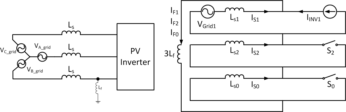
From the three-phase equivalent circuit, the positive-sequence equivalent circuit can be drawn. Only the positive-sequence circuit is considered because the three-phase fault is considered to be a symmetrical fault. Thus, the negative and zero sequence components are not present. The fault current contribution from the grid IF-GRID1 is limited only by the impedance presented by the inductance Ls1.
During a three-phase fault the three-phase voltage goes to zero. The three-phase currents are maintained at relatively constant values and allowed to be at Imax to contribute to the reactive power required to help maintain voltage without exceeding the current-carrying capability of the power semiconductors of the PV inverter. Note that with the three-phase short circuit, only the reactive current is considered because the output power that can be absorbed by the short circuit is near zero. In this example, the system protection is not activated. In many installations of PV inverters, system protection can be implemented to turn off the PV inverter after several cycles following the initial inception. The system protection setting is usually part of the fault ride-through requirement from utilities, so implementation may vary from one to another.
The grid contribution and the PV inverter contribution do not contain negative or zero sequence because of the nature of three-phase faults (symmetrical faults). Only during the beginning and end of the faults, small transient (negative- and zero-sequence) currents appear for both the grid and PV inverter contributions. Comparing the pre-fault to fault current, there is a significant jump of the short-circuit current (SCC) from the grid to the fault. The SCC from the inverter IINV1 is limited to Imax current controlled by the PV inverter.
Unsymmetrical Faults
The majority of the faults are unsymmetrical faults. They may involve the ground, such as SLG (n) and line-to-line-to-ground (LLG) faults, or they may be between two lines (LL) and not involve the ground. The short-circuit current contribution may also be impeded by the short-circuit current path to the ground. The zero-sequence current path is affected by the winding connections of the transformer and the generators. In general, any three-phase windings connected in delta or floating wye (Y) will block the flow of the zero-sequence current. Also, in some installations, the neutral (star) point of Y-connected windings is grounded via a small reactor (Zn) to impede the zero-sequence current.
Single-Line-to-Ground Fault
The most common type of fault is the SLG. This fault may be caused by a fallen tree on a single line, affecting only one phase. The other two phases continue to feed the loads. For loads insensitive to an unbalanced voltage, it will not affect the operation of the loads; however, for loads sensitive to unbalanced voltage (e.g., induction motors and generators), the unbalanced voltage may significantly impact load operation. A relay protection is usually used on the sensitive load to disconnect it from the grid in case a severe unbalanced condition is detected.
For an SLG, the sequence equivalent circuit consists of the series-connected positive-, negative-, and zero-sequence components of the network. To represent the PV inverter, a small modification is made to the sequence equivalent circuit. As the PV inverter is capable of generating symmetrical three-phase currents under normal and fault conditions, we have two switches (S2 and S0 are always open) to represent the absence of the zero- and negative-sequence currents in the PV inverter circuit. Thus, although the positive-, negative-, and zero-sequence currents are present on the grid side of the network, they do not show up on the PV inverter side. The impact of fault impedance (and neutral impedance) is multiplied by three to account for the fact that all the sequence currents (positive, negative, and zero) flow through this impedance. During a SLG the voltage of the faulted phase goes to zero. At the PV inverter, the three-phase output currents are maintained at a relative constant even during fault.
The grid SCC contribution contains identical positive-, negative-, and zero-sequence current, as is obvious from the sequence equivalent circuit for an SLG fault. The PV inverter contributions do not contain negative or zero sequence. The PV inverter can maintain symmetrical currents even during the fault. Small negative- and zero-sequence currents appear only during transition from normal operation to a short-circuit event. Comparing the pre-fault to fault current, there is a significant jump of the SCC from the grid to the fault. The SCC from the inverter IINV1 is limited to Imax current controlled by the PV inverter. Note that in the 3-LG fault condition, the fault current from the grid appears on all phases (a,b,c). In an SLG, the fault current from the grid appears only on the faulted line (Phase A). The SLG current is also quite large. As described previously, the fault current in Phase A for an SLG can be found as
\(I_{a-fault} = I_{a0}+I_{a1}+I_{a2}\)For an SLG, the fault current is
\(I_{a0} = I_{a1} = I_{a2}\) \(I_{a-fault} = 3I_{a0}\)To illustrate the impact of fault resistance on the SCC, 0.2 ohm was inserted to simulate the fault resistance. That leads to a significant reduction in the sequence current, by a factor of four. A similar technique can be accomplished by the insertion of neutral impedance on generators and transformers in the grid. The SCC from the PV inverter is not affected by the insertion of the fault resistance. Thus, the current controllability of the PV inverter does not change with fault resistance.
Line-to-Line Fault
A line-to-line (LL) fault may occur when lines are swinging and one line touches another. The swinging of the lines may be caused by wind, especially when the lines are sagging (possibly because of expansion during overloading). This fault may be cleared within cycles; however, it may persist, and the short circuit may be cleared by the circuit breakers after several cycles.
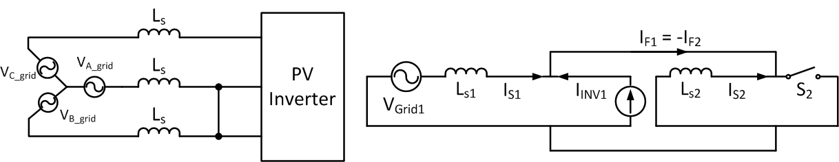
From the sequence equivalent circuit, the positive-sequence and negative-sequence equivalent circuit can be connected in parallel and drawn, which shows that only the positive- and negative-sequence circuits are considered. The LL fault does not have a zero-sequence component. Terminal voltage A and B are connected by the short circuit, and at the terminal voltage A and B are the same during the short circuit.
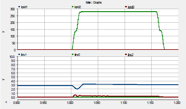
Figure on the right shows the grid voltage during normal operation and during the fault event. The grid voltage was normal when a sudden short between Phase A and Phase B occurred. As shown, at the point of fault incidence, Phase Voltage A and Phase Voltage B are identical due to the short circuit between them, but the voltages are not zero because there is no ground involved during the fault. The resulting voltage is represented by equal voltage, half the magnitude of the Phase A voltage, with the phase angle of 180° (the opposite polarity) with the voltage at Phase A. The positive- and negative-sequence fault currents from the grid are of the opposite polarity (IF1 = -IF2). The PV inverter current will not be affected because it will produce only a positive-sequence current. The negative-sequence equivalent circuit of the PV inverter is shown as the open switch S2 based on the fact that the PV inverter is capable of producing only positive-sequence currents.
The output currents of the inverter are not affected by the fault. The SCC contribution from the grid, as shown on the graph, is delivering short-circuit currents from Phase A to Phase B, as represented by two identical SCCs with the opposite polarity. Note that, although there is no fault current flowing to the ground, the SCC in the two phases (Phase A and Phase B) is much larger than the normal current. This current flows through lines A and B and through the winding of the transformers between the generator and the fault. If this fault persists, it must be disconnected from the grid to protect the power system components from overloading and overheating.
During a LL fault the positive- and negative-sequence SCC contribution from the grid is equal, and the zero-sequence component of the SCC from the grid does not exist as a consequence of the LL fault — the type of fault that does not involve the ground. The PV inverter is still producing the same output current in pre-fault, during-fault, and post-fault conditions.
Line-to-Line-to-Ground Fault
An LLG fault may occur when two lines are shorted to the ground. This fault may be cleared within cycles; however, it may persist, and the short circuit may be cleared by the circuit breakers after several cycles. From the three-phase equivalent circuit, the positive-, negative-, and zero-sequence equivalent circuits can be connected in parallel and drawn, which shows that only the positive- and negative-sequence circuits are considered. The LLG fault does not have a zero-sequence component. Terminal voltage A and B are connected by the short circuit at the terminals, and both of them are grounded. Voltage A and B are the same and equal to zero during the short circuit.
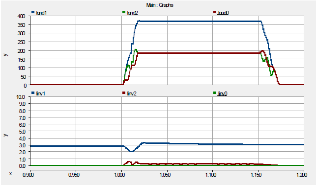
During a LLG fault the positive-sequence currents are almost double the negative-sequence currents, and the zero-sequence currents are almost identical to the negative-sequence currents. Of course, this current division between the zero and negative sequences can be altered by placing the neutral impedance on the zero-sequence path to reduce the size. The positive-sequence current will also be impacted by the neutral impedance. The PV inverter current will not be affected because it will produce only a positive-sequence current. The negative-sequence equivalent circuit of the PV inverter is shown as the open switch S2; the zero-sequence equivalent circuit of the PV inverter has an open switch S0, as the PV inverter is controlled to produce only positive-sequence currents.
Current Regulated Current Source Inverter
Another option to the CR-VSI is the current-regulated current source inverter (CR-CSI). The PV inverter uses the voltage Vgrid to synchronize the power converter to the grid by using the PLL to track the phase angle of the grid voltage. Thus, any changes in the phase angle or frequency will be followed as the power converter is locked to the grid voltage.
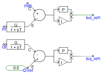
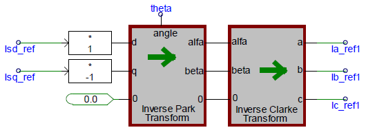
Control of the real power current component (IRE) and the reactive current component (IIM) can be easily implemented in the dq axis, with IRE represented by the q axis reference current Iq, and the IIM represented by d axis reference current Id. The PV inverter is capable of decoupling real and reactive power control. Real and reactive power reference signals are compared with actual values, and the error is used to drive two independent PI controllers. The real power error drives the Isd_ref signal, which is the current component in phase with the voltage (the real power component), while reactive power error drives the Iq_ref signal, which is the current component in quadrature with the voltage (the reactive power component). These dq0 domain values are the values of the current represented in synchronous reference frame synchronized to the grid. Thus, in steady state and in time domain, it gives constant values representing the magnitude of the real current component (Id_ref) and the magnitude of reactive current component (Iq_ref). The Idq_ref currents in synchronous rotating frame can be converted to reference Ia,b,c_ref values, expressed in stationary reference frame. (Note that the angle signal theta is calculated from the voltage phasor using the PLL block.)
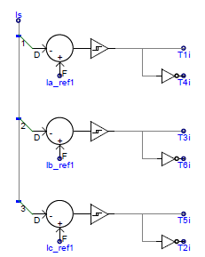
In stationary reference frame, this line current reference Iabc_ref takes the form of sinusoidal currents. The reference currents (ira-ref, irb-ref, irc-ref) are compared with actual currents, and a hysteresis controller switches the inverter IGBTs such that actual current follows the reference current. When the reference currents are achieved, reference real and reactive power are also achieved.
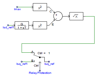
To limit the currents passing through the power semiconductor switches (e.g., IGBTs), a current limiter is used. When a fault (or severe undervoltage) is detected, the relay protection will signal the controller to switch to emergency mode. In this case, we want to produce the real power if possible but also generate reactive power with the remaining current-carrying capability of the IGBTs (< Imax) to support the voltage dip on the grid.
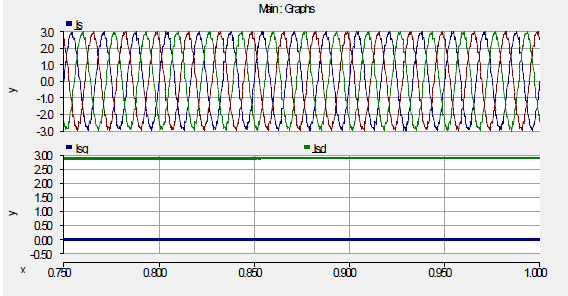
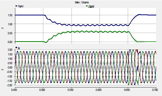
To test whether independent real and reactive power control have been achieved, real and reactive power tests were carried out by setting the real power to 1.5 MW and introducing an SLG fault. The SLG is introduced between 0.5 second and 0.65 second. As shown in Figure on the right, the real power delivered to the grid is 1.5 MW, and the reactive power delivered to the grid is zero during normal operation. Once the fault is detected, the reactive power can be delivered and is computed by calculating the remaining Isq_ref available to generate. As shown, the real power drops by about 33% because only two phases have normal voltage, so the normal phases (B and C) are able to deliver 66% of the rated power.
The reactive power generated is computed as 30% of the rated power. Note, that the d and q axis are in quadrature with respect to each other. Thus, the total current output is the phasor summation of Isq_ref and Isd_ref, and it is not an algebraic summation.
Grid Integration of PV Inverter
Historically, PV generation was developed on a small scale based on small PV modules (50 W–100 W). For a long time, PV modules were very expensive, and PV deployment was limited to isolated generation with battery storage. In early applications, the DC output was used to operate a radio, a light, or small tools. PV inverters were usually single-phase AC inverters at 60 Hz with output power less than 1 kW. Like any electrical appliance, small PV inverters are typically certified for safe application by Underwriters Laboratory (UL 1741). The certification emphasizes the safe use of this equipment.
As the adaptation of PV generation gained momentum, small PV modules were connected on the rooftops of residential houses. The size still was small, and the cost of PV modules still was high, so the level of PV penetration was not considered to have any impact on the power system at the distribution network. If there were to be any grid disturbances, these small PV inverters would disconnect from the grid and then reconnect after some time when the disturbance had ended.
The size of PV modules and PV inverters increased while the cost continued to decrease. There were a significant number of PV installations on the rooftops of commercial buildings. In many cases, the output power reached more than 100 kW. In 2003, the Institute of Electrical and Electronics Engineers (IEEE) issued IEEE Std 1547 to standardize the rules for connecting distributed generation (including PV inverters) to the distribution network. This standard was developed for low penetrations of solar PV in the grid.
IEEE 1547 is intended to ensure that renewable energy generation does not violate the basic rules of the distribution system. Conventional power flows from the generator to a residential load. With the increase of distributed generation such as PV generation, power flow may reverse direction when there is excess generation from, for example, a rooftop PV generating unit. Another concern is the safety of utility service engineers performing repairs in the distribution network because of islanding (when the PV generation keeps feeding local load after the circuit breaker disconnects the load from the main distribution network).
In addition, disconnection requirements dictate that distributed generation must:
- Cease to energize for faults on the area electric power system circuit
- Cease to energize prior to circuit reclosure
- Detect island conditions and cease to energize within 2 seconds of the formation of an island (anti-islanding).
PV inverter manufacturers strive to comply with IEEE 1547 [3][4], implement anti-islanding protection, and ensure that PV inverters stay connected within the allowable voltage-time and frequency-time operating region.
| Voltage Range and Maximum Clearing Time | |||
|---|---|---|---|
| Frequency Range and Maximum Clearing Time | |||
| Voltage Range (% Nominal) | * Max. Clearing Time (seconds) | Frequency Range (Hz) | Max. Clearing Time (seconds) |
| V < 50% | 0.16 | f > 60.5 | 0.16 |
| 50% < V < 88% | 2 | * f < 57.0 | 0.16 |
| V > 120% | 0.16 | ** 57.0 < f < 59.8 | 0.16 – 300 |
| 110% < V < 120% | 1 | ||
| (*) Maximum clearing times for distributed generation ≤ 30 kW; default clearing times for distributed generation > 30 kW |
(*) 59.3 Hz if distributed generation ≤ 30 kW (**) For distributed generation > 30 kW |
||
As the level of PV penetration continues to increase, fault ride-through capability (currently implemented for wind turbine generation) may be required for PV generation [5]. This requirement ensures that a wind plant is not disconnected from the grid at any fault unless the voltage at the point of common coupling lies beyond the voltage-time characteristic specified; thus, balance between generation and load can be maintained, and the cascading phenomena can be avoided.
As described previously, the PV inverter is generally placed between the PV module or array and the grid; thus, the PV inverter must process the entire generated power to the grid. There are two types of protection in solar PV inverters: fast disconnection (i.e., in less than one cycle) and continued operation for up to 10 cycles. The fast disconnection may be suitable for small PV installations connected to the grid or for isolated operations.
As summarized in [6], a PV inverter’s current contribution during a fault is not zero, and it varies by design. It was observed that, for most fault conditions, several PV inverters continued supplying current to the feeder subsequent to a fault for a period ranging from 4 to 10 cycles. The length of time the inverter supplies the fault current may be adjustable to comply with the regional reliability requirement. With reduced voltage, the output currents that can be supplied to the grid are limited by the current-carrying capability of the power electronics switches (i.e., IGBTs); thus, the output power is less than the rated power. If low-voltage ride-through is available, during the voltage dip, MPPT may be disabled to ensure the inverter follows the fault ride-through requirement rather than maximizing energy yield.
If the PV inverter is required to supply reactive power during the voltage dip, the PV inverter models may have to supply maximum reactive power available based on the current capability of the IGBT. The theoretical maximum reactive power contribution is when the voltage is leading or lagging 90 degrees. The PV inverter may be designed to carry short-term high current during the faults; many of them are designed to reach up to 120% or more of the rated current, depending on the customer request.
In some inverter models, the inverter current during faults was maintained at the pre-fault inverter current with this current setting, and the transition back to normal operation does not affect the PV operation drastically. Another mode of operation found in some inverter models is that the inverter current was dropped to 0 and the inverter was disconnected in less than 0.5 cycle for a fault when the terminal voltage reached less than 50% on any phase.
PV Inverter Model Validation
![]()
![]()
The PV inverter model was developed on the PSCAD platform. The general module of a PV inverter model was kept the same, but the control parameters and the system protection were tuned to represent the power inverter being tested.
This section is based on a collaboration between NREL and Southern California Edison (SCE). NREL developed the model for the PV inverter that was tested and validated in this paper. SCE provided the data for the dynamic model validation, which was developed on the PSCAD/EMTDC platform and created to model various PV inverters with flexibility in the implementation of different control algorithms. Although the PV dynamic model presented in this section was set to represent a specific power inverter tested at SCE, this model will be useful to simulate other PV inverters developed by different manufacturers with different control modules inserted to represent manufacturer-specific control algorithms and system protections.
Two types of faults were performed: SLG and 3LG. The response of the power inverter was recorded, and the simulation results were compared with the actual recorded data.
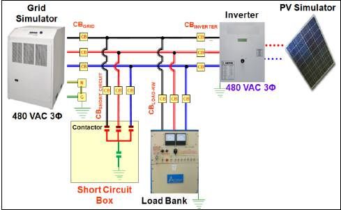
Bench Test Diagram
The bench test conducted at SCE is illustrated in Figure on the right. The grid simulator, load bank, short-circuit box, and solar PV were connected in parallel. The grid simulator was a programmable power supply that provided voltage reference for the inverter to start up. The PV simulator was a DC programmable power supply that allowed setting up the I-V curve for the solar PV inverter input. The load bank was to consume the power and balance it to zero. The short-circuit box was used to apply the short circuits for any given combination—symmetrical or nonsymmetrical, ground faults or non-ground faults. The data were captured within a specified time window—pre-fault, during the fault, and post-fault—to capture the transients and the action of the relay protection. A good reference on this subject can be found in reference [7].
Unsymmetrical Fault: SLG
The SLG fault was performed for this power inverter by closing one of the phases (A, B, or C) and the ground power contactors. For an SLG, the sequence equivalent circuit consists of the series-connected positive-, negative-, and zero-sequence components of the network. As the PV inverter is capable of generating symmetrical three-phase currents under normal and fault conditions, there is no zero- and negative-sequence currents in the PV inverter circuit, even during faults. Note that this behavior is different in voltage source generators such as a conventional synchronous generators.
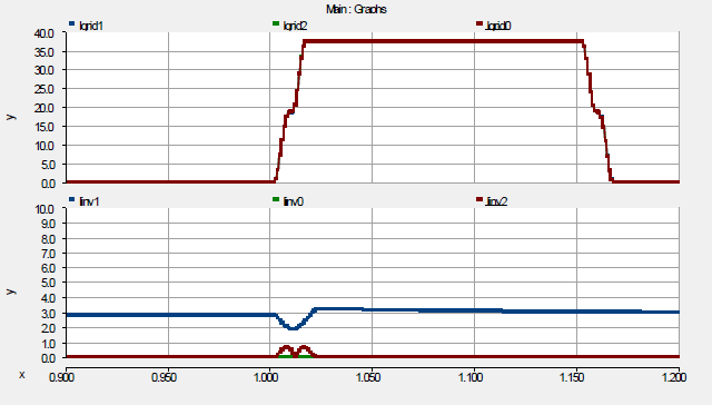
Phase Current Representation
An SLG, in which only one phase is shorted to ground while the other two phases are normal, is the most common type of fault. An SLG fault was simulated for this power inverter. The fault was a non-self-clearing fault occurring at t = 0.2 s. The power inverter was set to generate at a unity power factor, and the system was operating at 2.2 kW during normal operation (pre-fault). As a result, the real power dropped by one-third of the pre-fault condition and then fell to zero as the inverter tripped offline. There were oscillations in the real and reactive power that were a result of phase imbalance because the summation of the real and reactive power in the two active phases was not balanced. The reactive power stayed at zero before and after the fault.
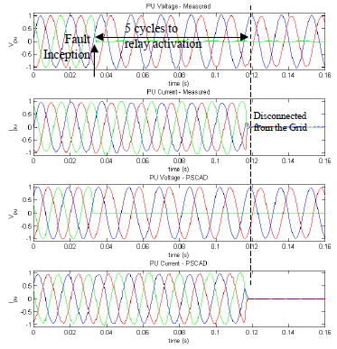
Comparison Between Simulation and Lab Experimental Data for an SLG
Figure on the right compares the measured and simulated terminal voltages and inverter output currents. The power inverter was set as follows:
- The output current was set at a unity power factor.
- The short-term maximum output current was set at 100% rated current.
The model relay protection was set to disconnect the power inverter after five cycles of low voltage (V < 50%) at any one of the phases.
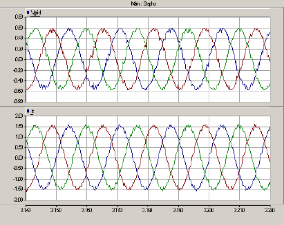
It is shown that the output currents are not affected by the fault because the PV inverter is controlled as a current source to supply the same fault current as the pre-fault condition.
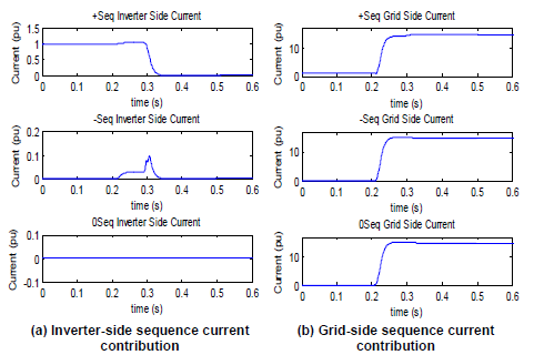
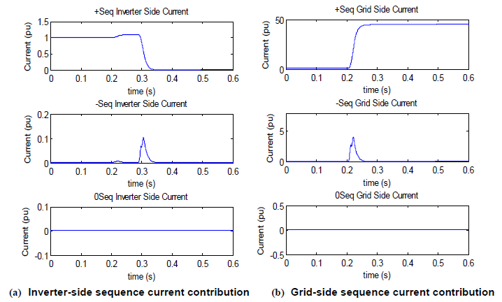
Sequence Current Representation
Figure on the right shows the comparison of the sequence currents between the line contribution and the PV inverter contribution. The normal current in the pre-fault region was very small compared with the short-circuit current contribution from the grid during the fault. During normal condition, the grid is always controlled to have a normal voltage (1.0 p.u.), thus behaving as a voltage source. During the fault, the fault current contribution from the grid is limited only by the line impedance. Line impedance is generally small; thus, the short-circuit current contribution from the grid is normally much larger than the rated current.
As the SLG is an unbalanced fault, it is expected that the output currents are unbalanced, with the faulted line current many times larger than rated current. The line contribution of the positive-, negative-, and zero-sequence currents appeared on the grid contribution to the fault. All sequence currents were equal in magnitude, as expected from an SLG fault. This is consistent with the assumed sequence equivalent circuit, where the grid side is represented by a voltage source in series with the sequence impedances (LS1, LS2, LS0). The PV inverter side is represented by a current source in series only with the positive-sequence impedance, while the negative- and the zero-sequence impedance is open circuit.
The PV inverter contributed only positive-sequence current, with a small negative-sequence (peak value at 0.1 p.u.) short-duration transient current. Thus, even in short-circuit conditions, the PV inverter output currents can be controlled to generate symmetrical three-phase output currents. Note that the PV inverter presented very large impedances to the negative- and zero-sequence currents. In the assumed sequence equivalent circuit, it is represented by the open switches in the negative- and the zero-sequence networks.
Symmetrical Fault: Three-Phase Fault
The 3LG fault was performed for this power inverter by closing the circuit breakers to the ground. The three phases were connected to the ground. Because this was a symmetrical fault, only the positive-sequence currents were present.
From the assumed sequence equivalent circuit, it is known that only the positive-sequence circuit is considered because the three-phase fault is considered to be a symmetrical fault; thus, the negative- and zero-sequence components are not present. Comparing the pre-fault to fault currents, there is a significant jump of the fault current contribution from the grid to the fault. The fault current contribution from the inverter IINV1 is a constant current controlled by the PV inverter; thus, the pre-fault output current will be the same as the fault current contribution from the PV inverter.
As expected, both the real and reactive power dropped to zero as all three phases dropped to zero. In this case, as in the previous one, the fault was a non-self-clearing fault, at t = 0.2 s, and the inverter tripped offline because of the severity and duration of the fault.
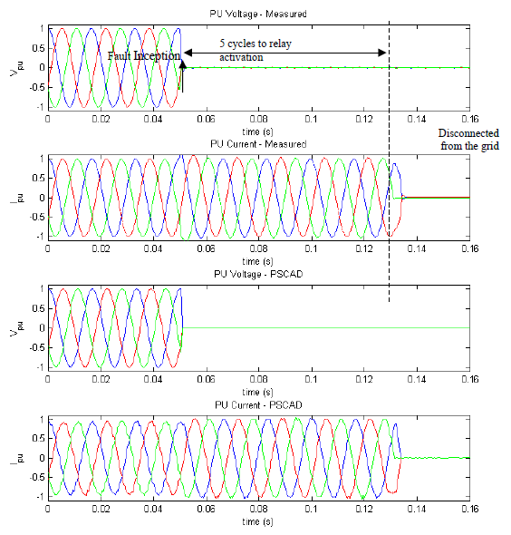
Comparison Between Simulation and Experimental Data for 3LG
Figure on the right shows the comparison between the simulation and the measured data. As shown, the simulation followed the measured data accurately, especially because the control system protection was set to follow the setting of the power inverter. The fault current in the three-phase output for this inverter was set to per-unit values. The system protection was controlled to let the current flow to the fault for the duration of five cycles after the fault, and once one of the phases reached its zero crossing point, this particular phase was deactivated. The other two phases continued to supply output current until they reached the zero crossing point. Then the last two phases were deactivated as well.
Because this was a 3LG, this was a symmetrical fault; thus, both the grid-side and the inverter-side short-circuit current contributions showed only the positive-sequence components. The negative-sequence components appeared for only a short duration during the fault transient, and the peak of the negative-sequence fault current is about 10% of the positive-sequence fault current. The zero-sequence currents are not shown because the value is very small.
It is worthwhile to note that the sequence current contributions from the PV inverter during the SLG and 3LG faults are identical; both contain only positive-sequence currents. The short-circuit current contributions from the grid are different for different types of faults.
Conclusion
This report described the development of a PV inverter model using PSCAD. We started with the fundamentals of the PV model at the solar cell by describing the I-V characteristic, the derivation of the equation, and the dependency of the output on the solar irradiance and the temperature. The equation for the solar array considered the fact that different PV inverters have different input (voltage, current, power ratings) specifications. Two types of MPPTs were implemented and simulated, and another MPPT was described.
The development of the PV inverter was covered in detail, including the control diagrams. Both the CR-VSI and CR-CSI were developed in PSCAD. Various operations of the PV inverters were simulated under normal and abnormal conditions. Symmetrical and unsymmetrical faults were simulated, presented, and discussed. Both the three-phase analysis and the symmetrical component analysis were included to clarify the understanding of unsymmetrical faults. This understanding about unsymmetrical fault operation is important because many PV inverters are connected to the distribution network, and most of the faults that occur are unsymmetrical faults, especially SLGs.
The dynamic model validation was based on the testing data provided by SCE. Testing was conducted at SCE with the focus on the grid interface behavior of the PV inverter under different faults and disturbances. The dynamic model validation covers both the symmetrical and unsymmetrical faults.
References
- ↑ NREL, PSCAD Modules Representing PV Generator, August 2013, [Online]. Available: http://www.nrel.gov/docs/fy13osti/58189.pdf. [Accessed March 2014].
- ↑ M. Cerroni, F. Mancilla–David, A. Arancibia, F. Riganti–Fulginei, and E. Muljadi, “A Maximum Power Point Tracker Variable DC-Link Three-Phase Inverter Control Scheme for Grid-Connected PV Panels” presented at the third IEEE PES Innovative Smart Grid Technologies (ISGT) Europe Conference (OCTOBER 14 – 17, 2012) in Berlin, Germany
- ↑ H. Tian, F. Mancilla-David, K. Ellis, E. Muljadi, and P. Jenkins, “A cell-to-module-to-array detailed model for photovoltaic panels,” J. of Intl. Solar Energy Society, vol. 86, pp. 2695–2706, Sept. 2012.
- ↑ A. Jain and A. Kapoor, “Exact Analytical Solutions of the Parameters of Real Solar Cells using Lambert W–Function,” Solar Energy Materials and Solar Cells, vol. 81, no. 2, pp. 269–277, 2004.
- ↑ D. L. King, “Photovoltaic Module and Array Performance Characterization Methods for all System Operating Conditions,” AIP Conference Proceedings, vol. 394, no. 301, pp. 347–368, 1997.
- ↑ D. L. King,W. E. Boyson, and J. A. Kratochvil, “Photovoltaic array performance model,” United States. Dept. of Energy, 2004.
- ↑ Keller, J. and Kroposki, B., “Understanding Fault Characteristics of Inverter-Based distributed Energy Resources,” NREL report number TP-550-46698, 2010.