Time Series Power Flow Analysis for Distribution Connected PV Generation

Author: Sandia National Laboratories^[1]

Distributed photovoltaic (PV) projects must go through an interconnection study process before connecting to the distribution grid. These studies are intended to identify the likely impacts and mitigation alternatives. In the majority of the cases, system impacts can be ruled out or mitigation can be identified without an involved study, through a screening process or a simple supplemental review study. For some proposed projects, expensive and time-consuming interconnection studies are required. The challenges to performing the studies are twofold. First, every study scenario is potentially unique, as the studies are often highly specific to the amount of PV generation capacity that varies greatly from feeder to feeder and is often unevenly distributed along the same feeder. This can cause location-specific impacts and mitigations. The second challenge is the inherent variability in PV power output which can interact with feeder operation in complex ways, by affecting the operation of voltage regulation and protection devices.

The typical simulation tools and methods in use today for distribution system planning are often not adequate to accurately assess these potential impacts. This report demonstrates how quasi-static time series (QSTS) simulation and high time-resolution data can be used to assess the potential impacts in a more comprehensive manner. The QSTS simulations are applied to a set of sample feeders with high PV deployment to illustrate the usefulness of the approach. The report describes methods that can help determine how PV affects distribution system operations. The simulation results are focused on enhancing the understanding of the underlying technical issues. The examples also highlight the steps needed to perform QSTS simulation and describe the data needed to drive the simulations. The goal of this report is to make the methodology of time series power flow analysis readily accessible to utilities and others responsible for evaluating potential PV impacts.

Introduction

Deployment of distributed PV systems is increasing rapidly. High penetration scenarios, which are becoming increasingly common, have the potential to affect the operation of distribution feeder equipment^[2]. The interconnection study process is designed to identify possible system impacts and mitigation alternatives. In the majority of cases, system impacts can be ruled out or mitigation can be identified without an involved study, through a screening process or a simple supplemental review study^[3]. For proposed projects that require a closer evaluation, existing methods, data, and simulation tools may not be adequate to fully characterize the potential system impacts. This report describes a time series power flow analysis method to fully characterize PV system impacts. The methods and assumptions discussed here could also be adapted to improve the way studies are done with existing tools.

Purpose of PV Integration Studies

A system impact study is performed to identify the potential electrical impacts associated with the integration of PV on the distribution system. The purpose of the impact study is to accurately identify adverse system impacts and determine options for mitigating the impacts. The need for better methods is not limited to interconnection system impact studies; it also includes the broader group of integration studies such as planning and operation studies. The types of impacts analyzed in a typical interconnection study are shown in table bellow.

Types of Impacts

Impact	Description
Voltage Regulation Device Operations	The change in the number of equipment operations by the devices that actively regulate voltage on the distribution system.
Steady State Voltage	The change in steady state service voltage delivered to the connected load on a feeder.
Voltage Flicker	End user voltage fluctuations that cause visible light flickers.
System Protection Analysis	The effects of DG current contribution on the coordination of protection devices.

Simulation Options

Commercial circuit analysis tools have historically provided the capability to analyze the power system at specific snapshots in time. More recently, simulation platforms have the capability to perform quasi-static time series (QSTS) simulations. Early QSTS tools like OpenDSS have been developed for research and academia, but new commercial circuit analysis programs now offer this capability. Some utilities and consultants are adopting simulation tools like OpenDSS and others like CYMDIST to perform more detailed studies.

For many years utilities have relied on commercial simulation tools to run steady state power flow and protection analyses on distribution feeders. The studies are limited to snapshots of critical time periods, such as peak and minimum load points which are selected to evaluate impacts on the distribution system. These simulations only provide a snapshot assessment of the powerflow on the distribution system and only give the magnitude of an impact at one instant in time. However, PV output is highly variable and the potential interaction with control systems may not be adequately analyzed with traditional snapshot tools and methods.

The main advantage of using QSTS simulation is its capability to properly assess and capture the time-dependent aspects of power flow. QSTS produces sequential steady state power flow solutions where the converged state of an iteration is used as the beginning state of the next. Examples of the time-dependent aspects of power flow include the interaction between the daily changes in load and PV output and the effect on distribution control systems. Another advantage of QSTS is the ability to analyze both the magnitude of an impact and also the frequency and duration of the impact.

The application of QSTS simulations requires more data to represent the time-varying PV output coincident with time-varying load. The time series data is often difficult to obtain as the measurement equipment at the feeder and PV plant will need to be upgraded with higher time resolution capability. The necessary data set can become very large depending on the resolution and length of simulation desired and simulation processing times can increase quickly and become burdensome. Details of voltage regulation controls, such as intentional delays, also need to be represented. If the simulation is performed in a simulation platform like OpenDSS that is different from the platform in which the data is maintained, the data conversion effort can be substantial. Automated conversion tools have been developed for certain platforms, but they are not readily accessible or require a significant amount of expert supervision.

QSTS Data

QSTS simulation introduces new and more complex data requirements for power flow simulation. The data requirements for QSTS can be divided into three categories: model data, load data, and PV data.

Most existing feeder models in present commercial software include large amounts of detail on the elements of the distribution system, including line definitions, transformer ratings, and details on other devices such as capacitors and voltage regulators (VREGs). The implementation of QSTS may require the gathering of additional system data including time delay control settings on voltage regulation devices such as capacitors and VREGs and more detailed information on the substation transformer and transmission source impedance.

QSTS simulations require the availability of historical time series load data and coincident PV output data. Time series load data is often not easily available at the required time resolution for the scenarios or study of interest. It is common for utilities to record feeder level load data at 15-minute or 1-hour resolution, but these time resolutions may be too low to analyze some aspects of PV system impacts. Since many of the time-dependent aspects on the distribution system, such as control time delay, function on the order of seconds it is necessary to synthesize high resolution load and PV output data typically at a resolution on the order of 1 second to drive the QSTS simulations.

For the examples shown here, 1-second time series data was generated by simple linear interpolation of the load data available at either 15-minute to 1-hour resolution. The load interpolation method is intended to set the base line for capturing the relative effects of adding PV. This method of estimating load assumes that load variability is relatively low compared to solar output variability. Using this method, the simulation will capture the long term, e.g. 15-minute, variability effects of load and also the short term variability effects due to PV variability. Obviously, load variability may not be negligible in some scenarios. The industry recognizes that high resolution load data is a gap that needs to be addressed going forward and many utilities are now collecting load data at higher resolution to address this gap.

Solar plant output time series data is typically not available for the specific scenarios of interest. Estimated PV output profiles need to be synthesized from either irradiance or proxy data from similar plants. Ideally, proximate time-coincident data should be used to capture the correlation of load and PV plant output. If actual or simulated time-coincident data is unavailable, performing QSTS using a basic diurnal PV output pattern could still provide some valuable insights. Irradiance data collection campaigns are increasingly being pursued for the purposes of understanding PV variability at the feeder level. Currently, EPRI leads a program to collect irradiance at various points along a feeder footprint and coincident load data. Entities like Sandia are developing and validating methods to generate reasonable PV plant output profiles (for individual plants and distributed PV) using irradiance. As more PV systems are being monitored, high resolution plant output data is increasingly available.

Estimating PV Power Plant Output

Photovoltaic impacts are driven by PV output; however, irradiance measurements are far more commonly available for a given location and timeframe. At 1-second resolution, PV output variability is related to, but not the same as measured irradiance variability; PV output directly relates to total irradiance over the plant footprint, whereas irradiance sensors are measuring only the local irradiance seen by small aperture sensor. The Wavelet-based Variability Model (WVM) is a method for estimating PV power plant output using an irradiance point sensor. The method basically scales variability at different time frames to account for the geographic smoothing that will occur over the area of the PV plant, which can correspond to a single PV system, or a collection of distributed PV systems^[4]. WVM was used for all but one of the PV plant output estimations described in the examples shown here to account for the spatial and temporal smoothing associated with the size of the PV plant.

Impact Analysis Method

This section highlights QSTS analysis examples on different feeders to describe methods that can be used for analyzing possible impacts of PV generation on voltage regulation. The examples included in this section cover the following three technical areas:

• Voltage regulation device operations
• Steady state voltage
• Voltage flicker

Each section includes a description of the impact, the analysis approach and method used, the specific reason for using QSTS, and an example illustrating the impact(s). All voltage references and results are relative to a 120 V base. All time references are relative to each feeder’s local standard time. Mitigation alternatives are also discussed for some impacts. As previously stated, the impacts of PV on a particular feeder are highly dependent on the specific situation. The example cases in this section are not applicable in general; they were intended solely to illustrate the various aspects of each method.

The OpenDSS simulation platform was used to perform the QSTS power flow simulations. Any electric power flow simulation with QSTS capabilities can be used with the methods and guidelines described in this section.

Example Feeder Models

Three radial feeders were used for the analysis examples. The general characteristics of each feeder are shown in table bellow. Historical load data at 15-minute or 1 hour interval was accessible for each feeder. The load for each feeder was allocated to each distribution transformer location, based on the transformer sizes. A power factor (PF) of 0.9 lagging was assumed. Since there are no line voltage regulators on any of the feeders, the Institute of Electrical and Electronics Engineers (IEEE) 8500 node test feeder was also utilized to investigate VREG impacts. High resolution irradiance or PV output data from a nearby location was used when the data was available.

General Feeder Characteristics

Feeder Attribute	Feeder-A	Feeder-B	Feeder-C	8500 Node
Load1	Peak: 7.5 MVA Min: 2.9 MVA	Peak: 3.5 MVA Min: 0.8 MVA	Peak: 1.7 MVA Min: 0.7 MVA	Peak: 11.1 MVA Min: N/A
Length (mi)2	3.36	3.05	3.54	10.56
Main Conductor Rating	630 Amps	552 Amps	274 Amps	Conductor Varies
Substation Transformer	115-20 kV 40 MVA FA	69-12.47 kV 14 MVA FA	46-12.47 kV 9.4 MVA FA	115-12.47 kV 27.5 MVA
Substation Transformer Load1	Peak: 33.2 MVA Min: 13.9 MVA	Peak: 4.7 MVA Min: 2.7 MVA	Peak: 4.1 MVA Min: 3.9 MVA	N/A
LTC Voltage Settings	120.55V, 3V Bandwidth, 30 sec delay, 6+j2 V LDC	121V, 2V Bandwidth, 60 sec delay, 7+j4V LDC	123V, 2V Bandwidth, 60 sec delay, 4+j3 V LDC	126.5 V, 2V Bandwidth, no delay, No LDC Not ganged
Load Class3	61% Commercial, 39% Residential	89% Residential, 11% Commercial	56% Residential, 44% Commercial	N/A
Capacitor Banks	900 kVAr Fixed; 2 – 1200 kVAr Switched (119.8V ON, 122.3V OFF, 30sec delay)	600 kVAr Fixed	300 kVAr Fixed	3- 900 kVAr Switched; 1 – 1200 kVAr Switched4
Voltage Regulators	None	None	None	3 Voltage Regulators
1 “Min” refers to the daytime minimum load found between 10:00 and 16:00. 2 Total conductor distance to farthest three-phase point from substation. 3 Transformers rated less than 125 kVA were considered residential, ≥125 kVA commercial. 4 Capacitor control: ON when the reactive power flow in the line is 50% of the capacitor size and switches OFF when the flow is 75% of the capacitor size in the reverse direction. Voltage override: ON at 0.9875pu and OFF at 1.075pu.

The Four feeder circuits figure shows the topographic layouts of Feeder-A, Feeder-B, and Feeder-C, and the IEEE 8500 node feeder.

Voltage Regulation Device Operations

There are three types of voltage regulation devices commonly used on distribution systems: load tap changers (LTCs), switched capacitors, and line voltage regulators (VREGs). The addition of PV may affect how these devices operate, depending on their operational settings, location and load level. Specifically, the issue of interest is whether PV generation materially increases or decreases the number of LTC and VREG tap changes and capacitor switching operations and how this impact may be mitigated. An increase of tap or switching operations does not constitute an impact that requires mitigation, unless the reliability or cost implications are deemed to be significant.

Device Descriptions and Operational Parameters

An LTC is an autotransformer used as a voltage regulation device on the secondary side of a substation transformer. LTCs are gang-operated devices that regulate the voltage according to a voltage setting, subject to a voltage bandwidth and time delay. The voltage setting may be adjusted seasonally or based on the load profile. The LTC typically has the ability to adjust the voltage ±10% with ±16 steps. Voltage is typically monitored on only one phase; however, the LTC action affects all three phases and all feeders at the distribution station. VREGs are essentially the same as LTCs, except they may be connected anywhere out on the feeder and are usually set to control voltage on each phase individually.

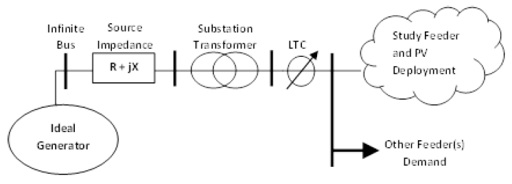
The purpose of the LTC is to ensure that steady state voltage delivered to all the connected load is within acceptable levels. The LTC source voltage is a function of the transmission voltage at the substation and the voltage drop across the substation transformer. Power flow studies on the distribution system assume that there is a fixed constant source voltage behind an impedance that represents the net impedance of all generators and transmission impedance to the substation. The short circuit current (SCC) at the substation can be used to represent the transmission system into a constant voltage source with an impedance calculated from the SCC. Because the LTC regulates the voltage at the substation, the LTC tap and the number of tap changes is only a function of the source impedance, substation transformer impedance, and net current flow, as shown in the Simplified Feeder Model Diagram. In the case of weaker grids (low SCC), it is especially important to model the source impedance accurately because changes in the load will significantly affect the LTC source voltage due to the high source impedance. Because the voltage drops across these impedances are current dependent, it is important to model the study feeder as well as all other feeders served by the substation transformer so that the total substation current is used to simulate the LTC source voltage. The addition of PV onto the feeder reduces the current across the circuit elements, therefore reducing the voltage drop across the elements. The change in voltage can affect the number of LTC operations, potentially increasing or decreasing the number depending on the case. The Simplified Feeder Model Diagram shows a simplified diagram of the feeder model with an infinite bus and source impedance calculated from the SCC for the transmission system connected to the substation.

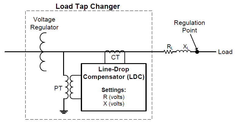
LTCs or VREGs may utilize a feature called line drop compensation (LDC). The purpose of the LDC is to allow for setting the voltage control point at a certain electrical distance downstream of the location of the LTC or VREG. This requires specifying the estimated electrical distance (expressed as an impedance R + jX) of the line segment between the LTC location and an estimated control point. The LTC operates based on the estimated voltage at the remote voltage control point. LDC is also especially useful for line voltage regulators, where the optimal location of voltage regulation on the feeder may present physical installation challenges and the LDC allows the regulator bank to be installed at a more ideal location nearby, while still achieving the desired voltage regulation.

The LTC with LDC responds not only to the voltage drop across the impedances of the transmission source and the substation transformer, but also to the voltage drop across the impedance of the section of line to the remote control point. Since the defined LDC impedances add to the combined impedances of the source and substation transformer, a change in current caused by PV has a greater voltage impact when LDC is employed.

For VREGs, the response to PV power production is essentially the same as for the LTC. An additional factor is that VREGs are not only affected by the current reduction due to downstream PV generation, but they are also affected by the change in the feeder voltage profile due to PV generation. If a large enough PV generation is connected downstream from a VREG, it may cause reverse current through the VREG. It is important that the VREG controls be set to properly handle reverse current.

Switched capacitor banks may also be used for voltage support with voltage set points defining when they are energized and de-energized, and other settings defining the switching time delay. Switched capacitors set for voltage support are affected by the change in the voltage profile of the feeder resulting from the addition of PV. If the switched capacitors are set for PF support, they are also affected by the change in measured PF on the feeder caused by PV displacing active power from the source.

Impact Concerns and Analysis Methods

The concern for voltage regulation devices is that a significant increase in the number of device operations could result in accelerated degradation and/or the need for a more aggressive maintenance schedule.

QSTS analysis is necessary to accurately quantify the effects of PV on voltage regulation device operations. The analysis should be an estimate of the long term, e.g. annual, difference in operations that can be expected due to PV. It is necessary to run both the base case and the PV case for comparison in order to quantify the impact due to PV.

The voltage regulation schemes on distribution systems can be complex with many factors to be considered including the devices deployed (LTCs, VREGs, and capacitors) and the location and control settings of each device. Coupling these factors with a unique deployment of PV, introducing its own factors of location, size, and variability, it becomes a difficult problem to identify a worst case period to study. In addition, the worst case period for one device may not coincide with the worst period for another. Identifying appropriate periods to study for the many possible scenarios is a complex process that will likely rely on engineering judgment. However, the examples in this section provide insight on identifying critical periods that may be useful in similar cases. The longer the study period, the better the long term estimate of operations. For any study period shorter than one year, it may be desirable to make a conservative estimate based on a worst case period.

It is also critical to properly simulate the behavior of the control algorithm of each device. All of the voltage control devices represented in the examples use a time delay setting, which determines the amount of time a voltage deviation can occur outside a specified range before action is taken to bring the voltage back within range. It would not be feasible to simulate this control behavior with snapshot analysis. Since typical control delays on VREG equipment are on the order of 30 seconds, a 1-second time step is recommended. It may be possible, depending on the variability of PV output and load, and the length of control time delays, to obtain similar results using a longer time step in the simulation. Because the goal of this method is to quantify the impacts in terms of the difference between the PV and no PV scenarios, using synthesized load data should yield reasonable results.

It is very important to properly model the correct regulator and capacitor control settings to get accurate results and to understand how the powerflow software platform used for the simulation implements control delays and the reset of delay counters. The time delay counter is triggered when an “out-of-band” voltage condition occurs. One approach is to set the timer to simply count up to the delay setting, and either take corrective action or not, depending on whether the voltage at the end of the counter is out of band or within band. This approach does not take into account the changes in voltage during the time delay count. Another approach is to use a sequential mode, where the time delay is reset if a voltage excursion returns within band before the duration of the time delay, only requiring action if the voltage remains out of band for the entire duration of the time delay. Most modern controls for VREG equipment and capacitor banks offer alternative modes of operation, such as voltage averaging and time-integrating. These control implementation options can make a difference in the way PV affects tap switching operations; therefore, it is important that the correct control settings be determined and properly implemented in the simulation software.

Example 1: Analysis of LTC Regulation Device Operations

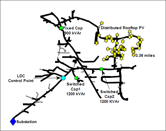
Feeder-A was simulated to illustrate the method for analyzing voltage regulation device operations. Feeder-A has an LTC at the substation with LDC and two switched capacitors. Feeder-A was modeled using coincident load and PV output derived from local irradiance data.

Example 1 Details

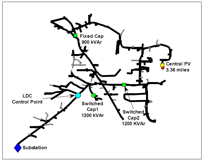
Feeder-A was simulated with a central PV system connected at the furthest three-phase point on the feeder that could thermally support the PV plant. The Example 1 figure shows the feeder layout with major component locations highlighted, including the central PV system location for this case. The hypothetical PV plant has a nominal capacity of 7.5 MVA at unity PF output, which is equal to100% of feeder peak load. The simulation was run from January 1, 2011 through September 30, 2011. This was the longest period with available time-coincident load and local irradiance data. The PV plant output estimate was derived using the WVM with local irradiance data at 1-second, assuming an area of approximately 62 acres at a density of 30 Wdc/m².

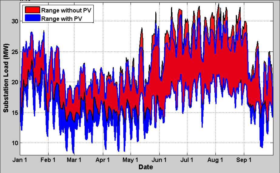
During the daylight hours with PV generation, a 1-second time step was used to capture the effect of PV output variability. For all other modeling periods without PV generation, including the base case without PV and night time hours, a 30-second time step was used. We verified that the 30 second time step did not affect the base case results. The Impact to Feeder-A’s substation load figure shows the 9-month power profile of Feeder-A’s substation load when adding the 7.5 MVA PV plant.

A comparison of the operations of the LTC and both switched capacitors for the 9-month simulation are shown in table bellow for the base case and the PV case.

Device Operation Comparisons, Base Case and PV case, 9-month Simulation

Device	Operations Base Case	Operations With PV (Differential)	Percent Change
LTC	459	394 (-65)	-14%
Cap 1	12	6 (-6)	-50%
Cap 2	16	28 (+12)	+75%

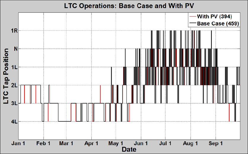
The addition of PV resulted in a net reduction in operations observed over the 9 months for the LTC and Cap 1 (nearest the substation), and an increase in the operations for Cap 2. The Feeder-A substation LTC is a ±8 step device, unlike the more common ±16 step devices, which means that each tap change results in twice the voltage change per step. Compared to a ±16 step device, we would expect that a ±8 step device would experience fewer operations. The LTC Operations: Base Case figure shows overlap plots of the device operations, base case and PV case, for the 9-month simulation.

The LTC Operations by Month figure on the right shows a column plot with the total LTC operations by month for the 9-month simulation for both for the base case and PV case. The differences shown in that figure highlight the periods where PV causes the greatest decrease in operations which is during the summer months and a small amount of additional operations which occurs in the winter months.

With the number of factors to consider on Feeder-A, it would be difficult to identify a period such as a week or a month that would have served as a feasible basis for long term estimation of the operations on each device. Periods with the greatest daily load swings from minimum to maximum will contain the greatest number of voltage regulation operations, which may result in periods susceptible to the greatest impact from PV. It may be prudent to take a closer look at specific days where there were increases, or decreases, in operations in order to understand the mechanism that results in impacts. A closer look at critical periods could also provide a basis for designing mitigation options, including adjustment of LTC control parameters.

Example 1A: LTC Decrease and Increase Operations with PV

Wednesday, June 22^nd is used as an example of one of the days where PV resulted in less LTC operations and Saturday, January 22^ndis used as an example of one of the “buck” days, where the PV caused an LTC buck operation. The power profiles include Feeder-A load, total substation load, and the PV power output for the PV case.

Because of the net reduction in LTC operations with PV over the 9-month simulation period, days during the peak load months in the summer like June 22^nd are very common. The loads and voltages for June 22^nd and January 22^nd figure illustrates the PV output reducing the voltage drop across the substation with LDC, which mitigated one of the midday boost operations, and in turn the buck as the load decreased near midnight. Both 1200 kVAr switched capacitors remained off in both the base case and PV case.

Saturday, January 22^nd is used as an example of one of the “buck” days, where the PV caused an LTC buck operation. The loads and voltages for June 22^nd and January 22^nd figure shows a comparison of the substation voltages, highlighting the LTC operations. The voltage profiles were taken from the same bus the LTC references for control. This figure illustrates the PV output reducing the current across the substation elements, thus reducing the LTC and LDCvoltage drop compensation. This resulted in a LTC buck operation at just before noon. Larger LDC impedance settings increase the likelihood that LTC operations will be impacted by the addition of PV. This also resulted in the need for a boost operation after the PV output has gone to zero at around 19:00. Both 1200 kVAr switched capacitors remained off in both the base case and PV case.

The LTC Operations: on June 22^nd figure on the right shows the LTC tap positions on June 22nd and highlights the LTC operations that were avoided due to the PV voltage support on the feeder.

Example 1B: LTC Increased Operations with PV – Boost Day

Monday, April 11^th through April 12^th is used as an example of one of the “boost” days, where the PV caused an LTC boost operation. The Feeder and Substation Loads and feeder voltages for April 11^th and 12^th – upper figure shows the base case power profile for Feeder-A load, total substation load, and the PV power output for the PV case on April 11^th and 12^th. Feeder and Substation Loads and feeder voltages for April 11^th and 12^th – middle shows a comparison of the substation voltages, highlighting device operations, on April 11^th and 12^th.

Feeder and Substation Loads and feeder voltages for April 11^th and 12^th – middle illustrates the PV output reducing the current across the substation elements, thus reducing the voltage drop across the substation and also reducing the LDC compensation voltage calculation. It also shows a case where PV output avoids a switched capacitor operation, visible at approximately 12:00 of the first day for the base case. This is due to the voltage change on the feeder caused by PV. Since voltage controlled switched capacitors only use the reference voltage at their location, and they are located out on the feeder closer to the PV location, they are more directly affected by the voltage rise effect. The further out on the feeder and larger the PV, the greater the voltage swings. The mitigation of the switched capacitor operation resulted in the need for a LTC boost operation in the case with PV once the PV output went to zero and the load surged in the evening around 19:00. This also resulted in the need for a buck operation as the load went down around 03:00 on the second day. Capacitor 2 remained off in both cases.

Feeder and Substation Loads and feeder voltages for April 11^th and 12^th – lower shows a comparison of the LDC point voltages, with device operations highlighted. Since the voltage in the Feeder and Substation Loads and feeder voltages for April 11^th and 12^th – lower is measured out on the feeder at the LDC control point, the relative variability and voltage rise from PV is greater. It is evident that the voltage rise mitigated the operation of Capacitor 1. This resulted in a chain reaction causing two extra LTC operations with PV.

Conclusions for Example 1

Example 1 illustrates the complexity that can be expected with the introduction of PV into a voltage regulation scheme designed primarily for unidirectional power flow. The combination of the reduction of current at the substation, as well as the voltage rise, can have a measurable impact on the operations observed. The use of LDC increases the complexity and impact further. The results of every case will be at least slightly different, since every voltage regulation scheme, feeder topology and PV scenario is different. QSTS analysis is necessary to properly model the interactions and accurately analyze the potential impacts.

An increase in switching operations alone does not necessarily represent a limitation on the amount of PV that a feeder can accommodate. All devices like LTCs with mechanical switching have a maximum operational lifetime and increasing the number of switching operations can decrease the lifetime of the device. However, the impact of an increase in switching operations can be mitigated by adjusting the LTC control set points to reduce the number of operations as shown in Example 1. A second mitigation may be to change the maintenance schedule to offset most if not all of the additional degradation of the device. It is unclear how much additional switching is required to cause accelerated degradation of the LTC, but prudent usage of the mitigation options should limit the negative impact.

Note that the distribution system in Example 1 is connected to a stiff 115 kV transmission system. This means the number of LTC operations will be lower than an LTC connected to a weaker grid (low SCC) or a lower voltage. The LTC for Feeder-A is connected to three additional distribution feeders, so the individual feeders may not change the substation current considerably. This explains why such a high penetration of PV on one feeder did not have a substantial impact to the number of LTC operations. PV variability can have a more significant impact on distribution system LTC’s for a weaker grid when the substation voltage fluctuates more with changes to the load and when there are fewer feeders on the transformer so that one feeder has more impact.

Example 2: Analysis of Line Voltage Regulation Device Operations

The IEEE 8500 node test feeder was used to illustrate the operations of VREGs with PV. The IEEE 8500 node test feeder has one set of VREGs at the substation and 3 sets of VREGs out on the feeder. There are also four capacitor banks. A 2 MW central PV system located just downstream from the first regulator was used as the PV scenario. This example did not utilize the WVM for PV output estimation, but rather proxy measurement data from a PV plant of similar size. The placement of the PV, regulators, and capacitors on the test feeder are shown in the IEEE 8500 Node Test Case with 2 MW Solar PV figure.

This analysis focuses on the VREG just upstream of the PV plant. From top to bottom, the IEEE 8500 Node Test Case Input Data and Results figure shows the feeder load and PV output, the voltages at the VREG with and without PV, and the increase in LTC operations with respect to the base case, shown as a running total.

The case with PV experiences a larger number of voltage variations due to the variability of the solar PV (middle chart). The bottom chart shows the importance of analyzing VREG banks by phase, since each one operates independently. VREGs, like capacitor banks, reference voltage at their location and are more susceptible to the greater voltage swings caused by PV output. This is seen in the running cumulative total of regulator tap operations for PV with respect to the base case.

Due to the phase unbalance in the feeder, aggregation of PV, and load variations, Phase-B experienced considerably more tap operations with PV than the other phases, with a total increase of 10 tap operations. On the other hand, Phase-C experienced fewer less tap operations with PV during the middle of the day than the other phases. This highlights the importance of not only considering the time-varying nature of the load and PV, but also the inherent unbalance associated with most distribution systems.

Example 3: Analysis of Mitigation for Excessive LTC Operations

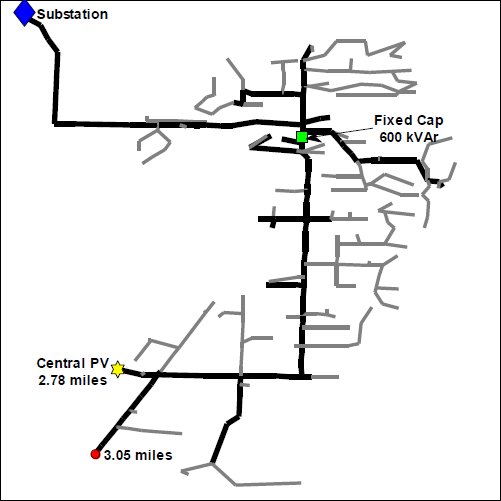
Feeder-B was used to illustrate how changing the LTC control time delay can reduce regulation operations. Feeder-B has an LTC at the substation with LDC and one 600 kVAr fixed capacitor. Feeder-B exhibits a substantial increase in LTC with the addition of PV.

The Example 3 Feeder-B figure shows the feeder layout with major component locations highlighted, including the central PV system. The LDC control point is not shown in this figure because the LDC setting for this feeder corresponds to an impedance point beyond the edge of the feeder. LDC settings such as this are not uncommon when multiple feeders of varying lengths are controlled by one substation LDC.

This analysis assumes a scenario with a central PV system connected at the furthest three-phase point of Feeder-B. At that location, the feeder ampacity is able to support a 3.5 MW PV plant (100% of feeder peak) at unity PF output. The PV plant output was estimated using the WVM with plant output data derived from 1-second irradiance data, assuming an area of approximately 35 acres at a density of 25 Wdc/m². The simulation was run for the week containing the peak PV penetration point for the data available. The peak PV penetration point occurs when the ratio of instantaneous PV output to instantaneous feeder load is largest. The simulations were run at 1-second resolution.

To investigate the impact of solar variability on the feeder, it is important to simulate a day with large PV output ramp rates and high variability throughout the day. One method for detecting highly variable days is presented here. From the available irradiance data, a single highly variable day was selected and duplicated for the week. The Example 3 Feeder-B: Load, Substation Load, and PV Output figure shows the base case power profiles for Feeder-B load, the total substation load, and the PV power output for PV case during the study period from May 20^th through 26^th.

The substation only serves two feeders. In the study scenario, the PV output often exceeding the substation load. Issues beyond voltage and device operations caused by the substation reverse power were not analyzed. In the study scenario, the PV output often exceeded the substation load and for the modeling of the LTC, it was assumed that the LTC is not set for reverse power flow and does not change state when current goes to reverse power.

A net increase of 62 operations, or 370% above the base case of 23 operations, was observed with PV for the study week. The LTC Operations: Base Case and with PV figure shows a comparison of the LTC operations for the base case and with PV.

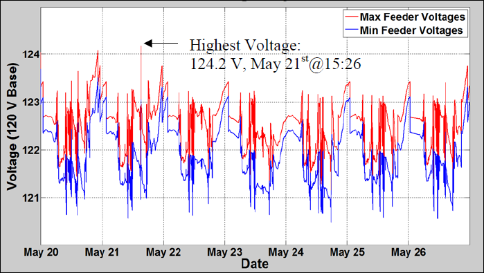
In this case, PV caused the need for several buck operations each day. Many of the operations were followed by operations in the reverse direction shortly after, in response to the PV variability during daylight hours. This analysis shows that a reduction in the number of operations can be accomplished by increasing the time delay of the LTC control. The original time delay setting of 60 seconds was increased to 90 seconds. Before increasing the control time delay setting, it would be prudent to make sure there are no voltage problems, because increasing the time delay may allow voltage to remain out of band longer than acceptable. The Maximum and Minimum Voltages figure shows the maximum and minimum voltages for the PV case simulation with a time delay of 60 seconds. The location of the max and min voltages varies during the simulation. All extreme voltages are within acceptable limits when the delay is increased to 90 seconds as shown in the Maximum Voltage Point Profile figure; therefore, no voltage issues are expected.

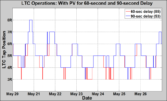
Increasing the time delay resulted in 53 LTC operations, a reduction of 32 LTC operations for the week from the 60 second delay. The LTC Operations: 60-Second and 90-Second Delay figure shows the LTC operations comparison for the 60-second and 90-second delay cases for the study week.

The 90-second delay eliminated several of the quick buck operations during the daylight hours by riding through the PV variability more often.

In summary, Example 3 shows that the base case of 23 LTC operations per week increased to 85 LTC operations with PV and a 60 second time delay and to 53 LTC operations with PV and a 90 second time delay. The increase in the time delay was very effective at reducing the net increase of LTC operations due to PV. There may be other impacts to investigate with a time delay increase, as well as other and/or longer study periods, but it is clear that this mitigation strategy can reduce the LTC operations with respect to PV variability if the change does not cause under /over voltages on the circuit.

Steady State Voltage

PV generation injects current into the system, resulting in a voltage rise at the PV Point of common coupling (PCC) compared to the voltage for the base case. The voltage change depends on both the current injection and impedance for the circuit path between the PV PCC and the nearest upstream voltage regulation device. The voltage difference between the voltage regulation device and the PV PCC is dependent on the direction and magnitude of the net current, the impedance and susceptance of the line, and the power factor. If the PV deployment level is high enough, a voltage rise will occur from the regulation point to the PV PCC. The PV Voltage Rise Concept figure on the right illustrates the concept of PV voltage rise for an overhead feeder with lagging load.

Feeder Voltage Overview

There are many factors that can vary the voltages on a feeder, including the transmission source voltage, substation transformer impedance, conductor impedances, distribution transformer impedances, load demand, load distribution and voltage regulation scheme. When PV is connected onto a feeder, it becomes another factor that will affect the voltage profile of the feeder, and ultimately the voltage provided to customers.

Distribution system operators in the US use the American National Standards Institute (ANSI) C84.1 as the operating envelope for acceptable steady state feeder and service voltage. The ANSIvoltage ranges shown in table bellow are for service voltage to systems at 600 V or less, which is defined as the point of common coupling between customer and utility.

ANSI C84.1 Range A and B Service Voltage Limits (120-V Base)

Voltage	Range A (%nominal)	Range B (%nominal)
Upper Limit	126 (105%)	127 (105.83%)
Lower Limit	114 (95%)	110 (91.67%)

The standard specifies two voltage ranges: Range A applies to normal operations and Range B applies for short duration and/or abnormal conditions on the utility system. For Range B conditions, corrective measures must be taken by the utility within a reasonable time to return voltages to within Range A limits. Range A and B exclude fault conditions and transients. Transient voltages beyond these limits are addressed by other voltage standards such as ITIC and CBEMA.

Impact Concerns and Analysis Methods

The concern with integrating PV, if the generation capacity is large enough, is the possibility of sustained over- or under-voltages, outside the ANSI C84.1 limits. This condition needs to be mitigated to avoid causing customer utilization equipment failure and/or damage, and/or nuisance protection tripping. High voltages could also interfere with the utility’s conservation voltage reduction program and result in PV inverter tripping and loss of energy production from a PV system.

Because radial feeders have historically been designed for unidirectional power flow from substation to customer, the lack of “headroom” for voltage rise due to PV is a common concern. For example, on feeders utilizing staged VREGs to solve significant voltage drop problems, the upper voltage limit for the VREG is often set at the ANSI A limit of 126 volts. Adding any additional PV systems downstream of the VREG can cause voltages to rise above ANSI range A due to the PV current injection at the PCC. The limited amount of voltage headroom available when using staged VREGscan often be mitigated by modifying the VREG control scheme while insuring that an acceptable ANSI voltage profile on the feeder is maintained.

In the case where LTCs or VREGs employ LDC, the addition of PV could cause low voltages on the feeder due to the de-sensitization of the LDC. When a PV system is connected downstream of a device employing LDC, the current injected into the feeder by PV will reduce the current across the device and reduce the voltage drop compensation which can potentially allow voltages lower than intended with the original settings. In the case of an LTC serving more than one feeder the presence of PV unevenly distributed among the feeders could make it more difficult to maintain adequate voltage regulation. This is because the feeders may have very different voltage profiles and the feeder with PV may see a voltage rise effect due to PV that may partially offset the change in voltage drop compensation.

Modeling

Because the voltage regulation scheme plays a crucial role in the voltage profile of a feeder, it is important to correctly model the feeder elements with the requirements specified here. In the case of an LTC employing LDC and serving more than one feeder, it is necessary to model all feeders served by the substation.

It is common practice to model only the primary voltage system without representing the secondary service drop to the customer meter, where the ANSI voltage limits actually apply. Since unidirectional power flow has largely been assumed, many utility planning models for feeders do not model the impedance of the secondary service drop and assume instead a conservative fixed voltage drop from the medium voltage side of the distribution transformer to the end of the secondary circuit at the metering point. However, a large enough PV system connected to the end of a secondary service can cause problematic voltage rises on the secondary service. Therefore if PV is connected to an existing secondary transformer that also contains customers, it is necessary to incorporate modeling of the secondary system for proper evaluation of the impact of distributed PV systems on customer service voltage levels.

Choosing the worst case study period within the available dataset for analyzing voltage concerns due to PV can be relatively simple in many cases. Because the voltage rise due to PV is related to the current output of PV, it is highly likely to find the time periods of the worst voltage increases when the ratio of PV system capacity to feeder minimum load is at a maximum. A more accurate method for choosing a study period when time series data is available is to determine the period of peak current injection relative to feeder load. This can be done by using the full data set of coincident loads and PV data points and subtracting them from each other at each time step to determine the exact time of peak PV current injection relative to load which should result in identifying the time with the worst voltage rise.

If LDC is employed and low voltage is a concern, the likely time to find the lowest voltages will be during a period of high PV output and high load demand. This is true because high PV output can desensitize the LDC and the greater the load demand, the greater the voltage drop across the feeder.

Since the voltage profile across a feeder varies, especially with complex combinations of voltage regulation and PV, it is important to locate the worst case locations for both high and low voltages with and without PV. For most overhead feeders without PV, the highest voltage point is at the feeder head and the lowest voltage point is somewhere at the end of the feeder. The end of the feeder can refer to either the end of the three phase backbone or to the single phase section depending on which circuit has the highest impedance path to the substation. When PV is incorporated, the highest voltage point on the feeder may shift to the PV PCC, especially for penetrations exceeding the feeder load, and the lowest point may shift to the end of another lateral, or even the feeder head.

Once a study period has been chosen the resultant voltage profiles for each point can be used for voltage analysis. Most utilities have traditionally used snapshot analyses to determine the existence of voltage issues, and the data collected for load demand is typically no higher than 15-minute resolution either averaged or instantaneous at each interval. The snapshot analysis approach tends to either overestimate or underestimate voltage issues depending on the data point used, and is unable to provide important details on the duration and frequency of voltage events. QSTS offers voltage analysis at high time resolution that is not possible with snapshot analysis tools.

Since ANSI does not apply to temporary voltage excursions outside the thresholds, it does not make sense to count a short-term excursion as a violation. Considering this, it is recommended that a moving average be used to calculate voltage profiles and to identify high voltage concerns when using data from high resolution QSTS analysis. The length of time for the moving average can be chosen to match the resolution of load data collection, such as 15-minutes, or set to shorter time frame for a more conservative voltage event estimate. The moving average will smooth the 1-second results of the simulation to determine voltage events/violations while still taking the effects of PV variability into account.

Steady State Voltage Analysis – Example 1

Feeder-A was simulated to illustrate the method for analyzing voltage regulation device operations. Feeder-A has an LTC at the substation with LDC and two switched capacitors. Feeder-A was modeled using coincident load and local irradiance data. The Feeder-A substation serves a total of four feeders, but the other three feeders were simulated only as a lumped load. Any voltage impacts on the other feeders were not included.

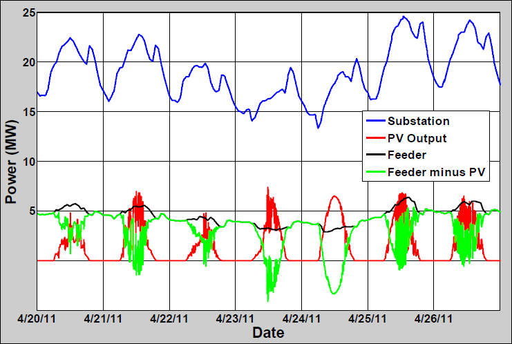
Feeder-A was simulated with several distributed rooftop PV systems on the secondary in an area at the end of the feeder that could support an aggregate nominal output of 7.5 MW (100% of feeder peak) at unity PF output. The aggregate distributed rooftop PV output estimate was derived using the WVM with local irradiance data at 1-second, assuming an area of approximately 232 acres at a density of 8 W/m². The simulation was run for a week surrounding Saturday, April 23, 2011 (included three days before and after) at 1-second resolution. The date was chosen for high voltage analysis, since the point of greatest reverse current for the data available occurred on April 23, 2011 at noon. The Example 1 Feeder-A figure shows the feeder layout with major component locations highlighted, including the interconnection locations of the individual distributed rooftop PV systems for this case. The Power profiles for April 20^th through 26^thfigure shows the total aggregate power output of the distributed rooftop PV systems at the end of the feeder in comparison to the substation and feeder real power.

The feeder model did not originally contain information on the secondary service, so a typical secondary service drop of 100 feet of 1/0 Aluminum Triplex was added to the model between the 120/240 V transformers and the load. The loads were modeled as 240V loads at the end of the triplex and the load allocation was at a 0.9 power factor. Each distributed rooftop PV system was connected at the load bus at the end of the secondary service line. The density of PV in the area chosen was modeled such that each individual PV system output was nominally just below 100% of its respective distribution transformer. This density of PV in this example was chosen to illustrate the potential secondary voltage rise that can occur.

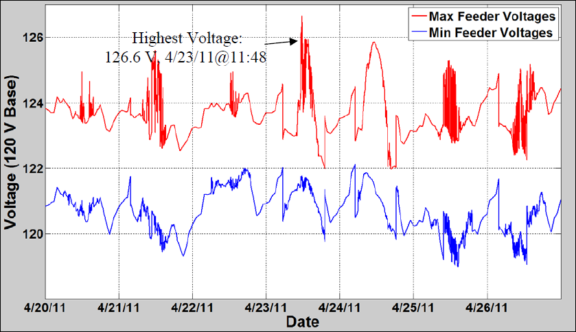
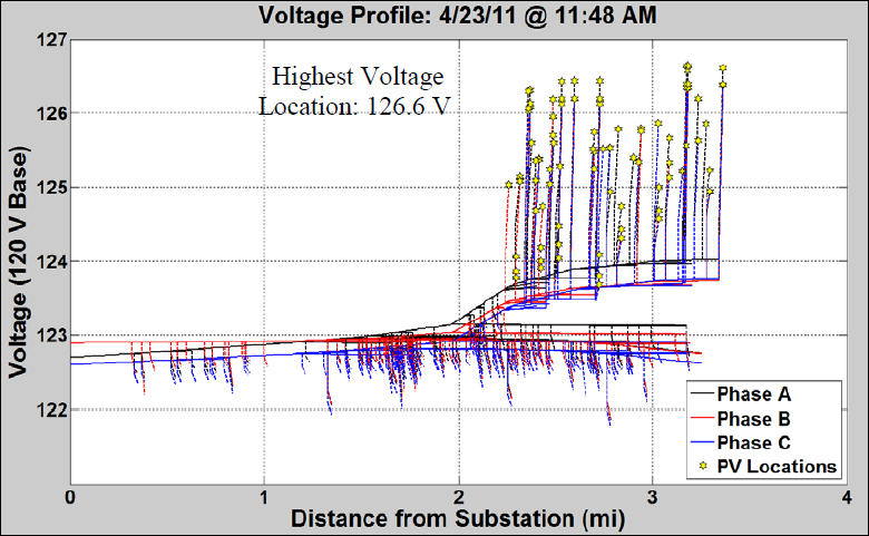
A check for voltage issues during the study week was performed as part of the QSTS analysis to verify the highest and lowest voltage found at any location on the feeder at each iteration. This allows for a thorough check to determine if further study is necessary and for identification of the location of the highest and lowest voltages, both with and without PV. The Maximum and Minimum Voltages figure shows the plot of the highest and lowest voltages for the PV case during the study week. this figure shows the time and magnitude of the highest voltage on the feeder. The Feeder-A Voltage Profile figure shows the feeder voltage profile at the time of highest voltage identified. This figure shows all phases and lines on the feeder, with secondary services shown as dashed lines. This illustrates the extreme voltage rise observed on the secondary with PV and the location of the highest voltage. A voltage monitor was placed at the bus serving this customer and the study week simulation was run.

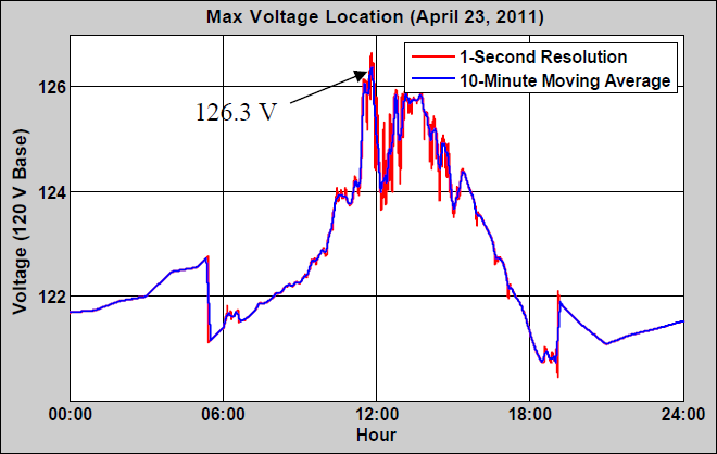
The one day of the study week that showed high voltages above ANSI C84.1 Range A (126 V) was April 23, 2011. The 1-second voltage profile is shown in red in the Maximum Voltage Location figure. The 1-second data was used as the input to a 10-minute moving average to create a smoothed voltage profile shown in blue. The 10-minute time period for time averaging is based on the ANSI C84.1 definition of voltage level. The smoothed voltage profile lowered the peak from 126.6 V to 126.3 V.

Example 1 illustrates the importance of considering secondary voltage rise to PV systems. It also illustrates the use of smoothing, making the tolerance similar to what has been conventionally practiced with SS analysis and load data resolution. QSTS analysis is necessary to properly capture the feeder interactions between PV variability, and load variability. QSTS is also necessary to obtain sequential results that can be used to determine the presence of an adverse impact.

Steady State Voltage Analysis – Example 2

Feeder-A was used for Example 2 to illustrate the method for analyzing the impact of PV output PF on steady state voltage as a mitigation strategy for high voltage issues. Feeder-A uses an LTC at the substation with LDC and has two switched capacitors. Feeder-A had coincident load and local irradiance data available.

Feeder-A was simulated with a central PV system connected at the furthest three-phase point on the feeder that could thermally support a 7.5 MW PV plant (100% of feeder peak). The simulation was run for the peak penetration week of April 20, 2011 to April 26, 2011. On over-voltage occurred on the fourth day of the simulation, April 23, 2011, and the analysis results focus this day, which is from hours 72 to 96 of the simulation. The PV plant output estimate was derived using the WVM with local irradiance data at 1-second, assuming an area of approximately 62 acres at a density of 30 W/m². The “IEEE 8500 Node Test Case with 2 MW Solar PV” inSection above shows the feeder layout with major component locations highlighted, including the central PV system location for this case.

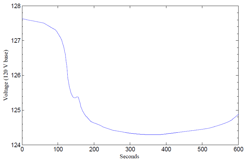
The left side of the Feeder-A Overvoltage Condition figure shows the maximum and minimum voltages anywhere on the feeder for each second of April 23^rd, demonstrating the range of voltages. The red line in this figure is the maximum feeder voltage plotted through time with the 7.5 MW PV plant at unity PF output. The maximum voltage occurs at 11:48:19 on April 23^rd, or hour 83.8 on the simulation hour timescale. The voltage profile plot along the entire feeder with the 7.5 MW PV plant is shown on the right side.

The goal is to enable deployment of high levels of PV on the distribution system without impact to customers. A common solution to the high voltage issues from PV is to adjust the power factor to absorb reactive power. The voltage decreases with even a slight change in the power factor to 0.95. Literature includes extensive discussions about the impact to the distribution system from absorbing volt-ampere reactive (Var) and changing the power factor on distributed resources and different possible power factor control strategies^[5][6][7].

To demonstrate the exact impact that the power factor of the PV output has on the distribution system voltage, the Voltage (pu) at the PV PCC figure shows the PV PCC voltage for the fixed instant in time (4/23/2011 at 11:48:19) for Feeder A with the 7.5MVA PV output at different power factors. With leading (absorbing) power factors, the voltage at the end of the feeder decreases, and with a lagging (producing) power factors, the voltage is increased.

Generally, as the PV output power increases, the voltage rises at the PV PCC because of impedance between the PV and the closest voltage regulation equipment. The PV PCC voltage is also a function of PV output power factor. An analysis of the PV PCC voltage as a function of both output power and power factor for Feeder A for 4/23/2011 at 11:48:19 is shown in the Voltage (pu) at the PV PCC as a function of PV output power and power factor figure.

Changing the voltage by adjusting the Var output (Volt/Var control) is prohibited by IEEE Std 1547 which stipulates that the inverter “shall not actively regulate the voltage at the PCC”. This means that the solar inverter is not allowed to directly measure voltage at the PCC and adjust its output accordingly. For this reason, Volt/Var control is not considered here. Other authors have studied how to implement Volt/Var control and the impact to the distribution system^[5][8]. Some authors^[9][10][11] have also investigated optimal distributed control strategies for the distribution system as a whole.

Other than the fixed lagging power factor previously mentioned, two other possible control strategies are proposed for adjusting the output power factor without directly measuring the bus voltage. The first power factor control strategy is to adjust the power factor by time of day. If from experience the distribution engineers know high voltages occur at specific times of day on the feeder, either from the solar output or the load, the power factor of the PV can be decreased during these times. This example simply decreases the power factor when the solar production is expected to be the highest in the middle of the day. The solar inverter could also be set to output Vars at certain times of day to support the voltage.

The same peak penetration week simulation for Feeder A was run with 7.5 MW PV plant at the end of the feeder, now with the power factor schedule shown in the figure on the right. The results in the Feeder voltages figure show lower voltages than when the PV plant is at unity power factor. The advantage of the power factor schedule is that in the mornings and evenings when the solar output is low, the solar output is at unity power factor, which helps support the voltage.

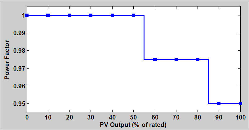
The second power factor control strategy shown is controlling the power factor as a function of PV output power. In the Example of power factor as a function of PV output figure, the PV PCC voltage is shown to be a function of PV output, so the PF can be designed as a function of PV output to counteract the voltage increase. Because a detailed simulation cannot be completed for every PV plant being installed, a generic function for power factor can be used. Similar to the concept for the power factor schedule, the power output is at unity power factor for lower solar outputs, which helps support the voltage. Some authors such as^[5] have proposed also making this a function of the X/R ratio at the point of interconnection.

The same peak penetration week simulation for Feeder A was run with 7.5 MW PV plant at the end of the feeder, now with the power factor function shown in the Example of power factor as a function of PV output figure. The results in the the figure on the right show lower voltages than when the PV plant is at unity power factor. The advantage of the power factor function is that it is directly proportion to the solar output, instead of assuming a certain amount of solar power at each time of day.

The three methods (fixed power factor, power factor schedule, and power factor function) are graphed together in the Feeder voltages with varying ways of modifying solar output power factor figure. Each of the example control methods brings the maximum feeder voltage for Feeder A within the appropriate limits.

The benefit of decreased high voltages or supporting low voltages is not without consequence. The solar inverter must stay within its kVA rating. For the simulations shown above, the inverter rating was assumed high enough to maintain the full solar output and the requested absorbing Vars. Under high solar output weather conditions, the reality is that an inverter rated for the PV system would have very little capacity left for producing or absorbing Vars. This headroom for reactive power output between the inverter rating and the real power solar output varies throughout the day as the solar irradiance varies. When a higher reactive power output is requested by the inverter control (fixed power factor, schedule, or function) than there is in the headroom of the inverter kVA rating, either the reactive power or the real power must be reduced from the specified conditions.

Voltage Flicker

Voltage fluctuations on electric power systems caused to various degrees by motor starts, PV variability, etc., can be large enough and frequent enough to give rise to noticeable changes in illumination from lighting equipment. This phenomenon is often referred to as flicker or voltage flicker. PV output ramps up and down during periods when there are moving clouds. The effect on voltage depends on the amount of PV and the location. Although PV induced voltage changes are typically well inside ANSI voltage limits, it is possible that under certain conditions, the frequency and magnitude of the voltage changes could drive a flicker impact. One way to establish whether voltage fluctuations are a concern is to compare the voltage profile with and without PV keeping all other factors the same. This is equivalent to a 100% change in power. If the difference is sufficiently small, no further study may be necessary. If the difference is significant, then the PV induced voltage changes should be evaluated to determine if they are objectionable according to established flicker limits.

The measurement of flicker involves a quantification of the system voltage variation and the frequency at which the variation occurs. The common metric for assessing light flicker has been to evaluate voltage fluctuations per the IEEE 519-1992 flicker curves (see Maximum Permissible Voltage Fluctuations figure). This figure shows voltage vs. frequency flicker curves based on historical data from incandescent lights showing how voltage fluctuations translate into visible flicker. The top curve represents the borderline threshold where flicker becomes objectionable. The bottom curve shows the borderline threshold where flicker is detectable by the human eye. The flicker curves have historically been used by utilities to evaluate the impact of square waveform voltage events such as motor starts and other types of loads that can be expected to occur with a certain frequency.

The IEEE 1453 recommended practice (IEEE Recommended Practice for Measurement and Limits of Voltage Fluctuations and Associated Light Flicker on AC Power Systems) supersedes the flicker curves and flicker limits in IEEE 519-1992. IEEE 1453 is a recommended practice that adopts the International Electrotechnical Commission (IEC) 61000-4-15 standard which defines both the measurement protocol and the functional specification for the flicker measuring apparatus or “flicker meter”. IEEE 1453.1 is a guide that adopts IEC 61000-3-7 standard for determining appropriate flicker planning levels and emission limits.

The disadvantage of using the older IEEE 519 flicker curves for evaluating the voltage variation caused by PV is twofold. First, the flicker curve requires knowledge of not only the percent voltage dip caused by variation in PV plant output but also the frequency of the voltage dip.

The frequency can be very difficult to quantify for cloud patterns that are not consistent. The second problem is the design of the flicker curve which was developed to address fast voltage changes such as motor starts and not the slowly changing voltage variation seen with PV. These problems with the IEEE 519 flicker curves often lead to an unnecessarily conservative approach for determining PV induced flicker impact. The IEEE 1453 recommended practice utilizes “mathematical functions to describe the flicker effects of any waveform envelope and is the best method for assessing PV induced voltage flicker.”

Key Aspects of IEEE 1453-2001

The IEEE 1453 recommended practice defines the two key metrics, P_ST and P_LT, to quantify the flicker disturbance level. P_ST is defined as a measure of short-term perception of flicker and it characterizes the flicker severity with one value obtained for each 10 minute period. P_LT is defined as a measure of long-term perception of flicker and it characterizes the flicker severity with one value obtained for the 120 minute period. This value is calculated using 12 consecutive P_ST values per the following formula

\(P_{LT}=\sqrt3{\frac{1}{12}\times \sum_{j=1}^{12}P_{LT_{j}}^3}\)

The voltage fluctuations limits on the medium voltage (MV) power system are shown in table bellow. MV is defined as nominal voltage greater than 1 kV and less than or equal to 35 kV.

Compliance levels for P_ST and P_LT for MV power systems

	Compatibility Levels	Planning Levels
PST	1.0	0.9
PLT	0.8	0.7

The IEC standard describes the probability levels used for determining the compliance levels. The compatibility level for flicker is based on a 95% probability level that there will be no complaints due to voltage fluctuations. The more conservative planning level for flicker is based on a 99% probability that there will be no complaints due to voltage fluctuations.

The methods to assess flicker include hardware devices, analytic methods and detailed simulations. The hardware method consists of using a flicker meter to measure, record and analyze the voltage variation signal. IEC 6100-4-15 gives the functional and design specifications for the flicker measuring apparatus or “flickermeter.”.

The analytical method evaluates voltage time series data by applying shape factors to quantify the flicker effect. The simulation method involves using software simulation of the flicker meter to analyze voltage time series data. The simulation method is the preferred method for evaluating flicker impacts of PV systems in an interconnection study because it is simpler to implement than the hardware method and offers a more detailed and rigorous analysis of voltage fluctuations than the analytic shape factor method.

Flicker Example Analysis

The need for a formal flicker analysis should be established by evaluating the effect of a 100% change in PV output. If further study is justified, then a time series simulation can be performed, and the resulting voltage profile can be evaluated against the IEEE 1453 criteria.

Implementing a detailed simulation of PV system output variation involves a choice between using irradiance sensor data to represent PV output or using estimated output of the PV plant taking into account spatial and temporal smoothing across the plant footprint. The latter method more accurately estimates PV plant output ramps, while the irradiance sensor only approach tends to overestimate ramp changes. Estimating the PV plant level ramp rates is very important to achieve the most accurate simulation of flicker impacts. The PV plant output estimate was derived using the WVM with plant output data derived from 1-second irradiance data at a similar location.

Feeder-B was chosen to illustrate the methodology. The feeder has the weakest source compared to the other example feeders in our study group and was found to have relatively large voltage changes per MW of PV. The studied system was a single 1.75 MW PV plant located on the edge of the feeder 3.44 miles from the substation. The PV plant capacity is 100% of the feeder peak load and 240% of the feeder minimum load. The large PV system size relative to feeder load was selected to best illustrate the flicker evaluation.

The observation period according to the IEEE 1453 recommended practice shall include the period of time in which the equipment under test (PV system in this case) produces the most unfavorable sequence of voltage changes. Determining the period of observation for a PV system presents two major challenges:

1. Determining the correct period of variability to study, and
2. insuring that voltage fluctuations caused by outside events not related to solar variability are either removed from the data set or accounted for by a comparison to a base case without PV. For this example we choose a 2 hour observation period with the largest voltage change ramp during a ten minute period. Although the largest voltage ramp criterion is unlikely to be the optimal method for determining the worst case flicker condition, it did identify a highly variable period to highlight how this method functions.

Results

A QSTS powerflow analysis was performed on the feeder and interconnected PV system and the voltage profile was recorded on the MV side of the PCC for the PV system. The voltage profiles show that a large percentage of the 1 second simulations are outside of ANSI A and B voltage ranges. The high voltage profile is the result of the voltage rise caused by the large PV system size relative to feeder loading. Since the flicker calculation is concerned with voltage differences and not absolute voltages, the high voltage profile does not impact the results.

The largest MW ramp during the 2-hour period was a 1.24 MW down ramp which occurred over a 5 minute period at a little over 1 hour into the 2 hour period. The large drop in MW caused by a cloud shadow resulted in a 3.3V change or 2.65% voltage drop at the PCC as shown in the Largest voltage change ramp figure. The short term voltage flicker calculated using the flicker meter for the large voltage ramp was measured with a P_ST = 0.07, which is well below the planning level of 0.9. This shows that the flicker associated with the largest delta V ramp, was not a problem for this feeder.

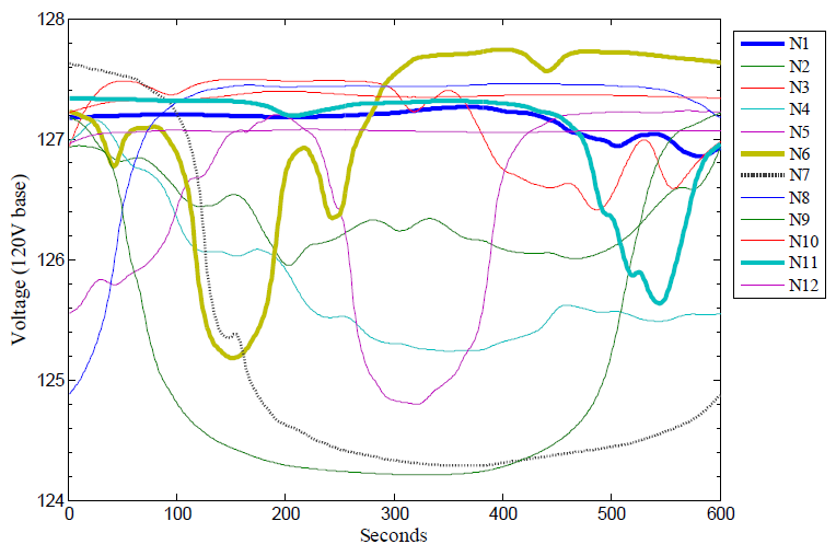
The 2 hour period contains many other voltage fluctuations caused by changing cloud shadows that can be evaluated using the long term flicker criteria P_LT. The Voltage profile at medium voltage level figure shows the twelve voltage profiles at the medium voltage level for each of the 10 minute periods. The voltage profile for the largest ramp is labeled N7 in this figure. Three other voltage profiles (N1, N6 and N11) are highlighted that have much larger P_ST values than N7, showing that flicker severity is dependent on both the rate of voltage change but also the frequency. See table bellow for the P_ST values for each voltage profile.

Summary of P_ST values for 12 voltage waveforms

Voltage Fluctuation Period	PST
N1	0.71
N2	0.14
N3	0.22
N4	0.05
N5	0.14
N6	0.61
N7	0.07
N8	0.04
N9	0.04
N10	0.06
N11	0.79
N12	0.07

Three of the ten minute periods have P_ST values approaching the 0.9 planning limit. The voltage profile for each of these periods indicates that a better way to choose the time period for maximum flicker impact would be to concentrate on the periods with the most rapid changes in voltage.

The P_LT value for this two hour period is 0.45 which is well below the 0.7 planning limit showing no long term flicker problem. The exact two hour time window picked for observation will affect the P_LTvalue, but does not change the result that no flicker impacts are expected for this very large PV system on the outer edge of feeder with a weak feeder source.

Conclusions

PV induced voltage fluctuations are slow to change over many tens of seconds and it therefore takes significant PV plant output changes for the flicker to be observable on the electric power system. This example demonstrates a method for evaluating flicker using the IEEE 1453 standard and demonstrates no flicker problems on the feeder with a very high PV deployment level.

Implementing this method is data intensive, but the data needed matches the data required for the other QSTS analysis examples discussed earlier in this report. The primary benefit of using the IEEE 1453 method for flicker evaluation is the significant increase in accuracy compared to the IEEE 519 “snapshot” methodology.

Flicker may become an issue for PV on distribution systems where the interconnection point on the feeder results in a high impedance path back to the feeder source and when PV deployment levels are high. Determining the appropriate PV deployment capacity threshold for flicker issues as a function of the interconnection location and other meaningful feeder specific metrics is the subject of ongoing research and development.

Fault-Current Analysis

Power system faults such as short circuits will occur on even the best designed and maintained distribution systems, so utility protection systems must be designed to clear faults by interrupting the source(s) and after the fault is cleared restore service to as many customers as possible. The basic element of utility distribution system protection against short circuit faults is time-overcurrent relaying. Since relaying can be adversely effected by fault current sources distributed throughout the feeder, it is very important to know the short circuit fault current levels throughout the system.

The design of overcurrent protection for radial distribution systems is based on the principle that power and fault current will flow from the substation source out to the loads and faults and that there are no other sources of fault current. The interconnection of PV inverters to the distribution system introduces new sources of fault current that can change the direction and magnitude of fault current flow and also introduce new fault current paths.

Fault circuit analysis is focused on determining the magnitude of the fault current along the feeder so that an interrupting device such as a circuit breaker, recloser, sectionalizer or fuse does not see fault current exceeding the device’s interrupting capacity. Determining the fault current magnitude is also required to insure protection coordination so that the device(s) interrupting the fault are the ones that minimize loss of load on the feeder. Finally, fault current magnitudes are required to insure that clearing times for protective devices are sufficient to avoid feeder equipment damage such as conductor overloads for end of line faults.

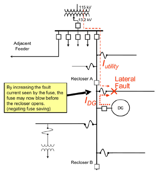
The Potential Coordination Issue for Fuse Saving figure illustrates a potential coordination issue where the addition of PV fault current can reduce the effectiveness of fuse saving schemes. The fuse saving scheme shown in this figure depends on the recloser upstream of the fuse to clear a temporary lateral fault before the fuse blows. A PV system located downstream of the fault location may negate fuse saving by feeding the fault as a second source and increasing the fault current seen by the fuse, which blows the fuse before the recloser can open.

The Potential Coordination Issue for EOL faults figure illustrates another potential coordination issue where the addition of PV fault current can reduce the feeder breaker’s zone of protection and limit the breakers ability to see end of line faults and thereby leave sections of the circuit without overcurrent protection. The normal setting for the breaker in this figure, without any DG, is for the breaker to provide over current protection for all faults on the feeder including the end of the feeder shown at point R. The breaker relay is set so that the total fault current through the breaker for an end of line fault at point R is sufficient to trip the breaker. A PV system located midpoint on the feeder will inject fault current for an end of line fault which results in a lower fault current seen by the breaker relay. The breaker relay becomes de-sensitized by the PV fault current injection and the breaker’s zone of protection now ends at the point Q. If the breaker settings are not adjusted, the addition of PV fault current can result in feeder conductors and other equipment being exposed to over-current conditions for faults downstream of point Q.

Other important protection coordination issues beyond those described above are sympathetic tripping of adjacent feeders and the addition of multiple new ground sources and ground fault paths due to numerous PV connections.

The need to involve accurate models of all the distributed generation on the circuit and the distribution system components seems obvious. However, fault studies for radial systems without DG rely on the fact that the vast majority of loads do not provide fault currents. For this reason, distribution transformers and secondary circuit impedances are not modeled, even when the software can do so. In situations where additional fault current from PV connected on customer premises is a concern, inverter fault current contributions may need to be taken into account, and modeling the distribution transformer and secondary circuit impedance may be necessary. If present, distribution-connected synchronous and induction generators, along with their associated transformer impedance and winding configuration, should also be modeled as well.

Generators and Inverters

The fault contributions provided by synchronous and induction generators will have a significant impact on both the fault withstand requirements of the equipment as well as the protective relaying design. There are well-accepted standard models for both synchronous generators and induction generators, although it can be difficult to obtain accurate parameters for smaller machines. However reasonable estimates can be made from typical machine values. The contribution from DG machines is generally a small fraction of the total fault current contributed by the utility bulk power source. An error in estimating the machine parameters often has only a secondary impact.

A common practice for computing the DG contribution to the fault is to model machines with a Thevenin equivalent voltage behind the direct-axis transient reactance (usually denoted as Xd’). This value is typical 25-30% on the machine’s kVA base.

Accurate fault models are not generally available for inverters and typical distribution system analysis tools do not have the capabilities to model the dynamic behavior of inverters and their controls during abnormal system conditions. In fact, active research continues regarding the appropriate performance characteristics for inverters during faults. Even if detailed inverter models were readily available and planning tools could accommodate them, distribution planners would be reluctant to use them due to the sheer number of variables required to populate the models. The detailed model approach will have to wait for the industry to provide packaged models that require little effort to incorporate into planning tools. In the meantime, planners will resort to average models for impact studies.

Different Approaches to Modeling Inverters for Impact Studies

One approach to modeling inverters for a fault study is to assume that the inverter does not provide sufficient fault current to affect the time-current curve coordination of the distribution system relays. This approach assumes the inverter contribution is negligible or that the inverter shuts off immediately when the fault occurs. At low levels of penetration of inverter-based DG, this has been a successful approach. Inverter fault detection schemes do a good job of shutting down for faults where the terminal voltages clearly indicate a problem. However, many faults occur on utility distribution systems where the voltages do not collapse completely and inverters continue to supply current. At high penetration levels, a better approach is needed.

A second approach to modeling inverters for a fault study is to assume inverters behave like similarly-sized synchronous generators during faults. A common practice is to assume that the inverter can be modeled by a Thevenin equivalent that will yield at most 2 pu current if a bolted short circuit were to occur at the inverter terminals. Thus, Xd’ assumed to be approximately 50% or larger, and the inertial constant is set very large so that the machine phase angle does not move much for the duration of the simulation. The idea is that this provides an upper bound on the short circuit current levels and if this does not have an impact on the short circuit protection coordination, it is acceptable. The value of 2 pu comes from research that indicates the initial pulse of current from the inverter can reach this magnitude when dumping into a bolted fault. Of course, this magnitude of current would cause the inverter switch protection to stop the inverter and it would not continue at this level. Persistent overcurrent magnitudes from inverters are typically in the 120% – 125% range. It is usually safe to assume that most inverters will voluntarily shut down quickly above this range to protect the switches from overcurrent. Underestimation of fault current contribution is possible with this Thevenin representation if the impedance is not changed to adapt to fault location and the resulting changes in inverter terminal voltage.

A third approach to modeling inverters for a fault study is to model the inverter by a Thevenin equivalent voltage source that is behind an equivalent impedance shown as Z1 in the figure on the right. The equivalent impedance is set to yield the maximum fault current specified by the inverter manufacture for a bolted short circuit fault and it depends on the magnitude of the inverter terminal voltage. If this is not done, the Thevenin equivalent may underestimate the fault current contribution for certain fault locations. The solution is to iterate through a couple of fault studies to find the correct Z1 to yield the maximum inverter output for the actual fault location on the circuit under study. It is often difficult getting accurate data from the manufactures about the maximum fault current and determining the time frame when the maximum was measured.

A fourth approach to modeling many grid-connected inverters is to assume the inverter current stays nearly steady until the terminal voltage drops so low that the inverter disconnects from the grid per 1547 trip thresholds. With this approach, the planner would assume that the current contribution increases to 110-120% of rated output after the fault occurs and remains constant until the inverter trips offline. This gives a conservative estimate of the potential impact of high penetration PV, for example, on the overcurrent protective relaying.

Conclusion

This report shows how new analysis methods using quasi-static time series simulation and high time-resolution data can better characterize the location specific impacts and mitigations for interconnecting high deployment levels of PV systems on the distribution system. The examples in the report demonstrate the usefulness of the new analysis approach for determining the effect of high levels of PV on distribution system operations. The report also illustrates new methods to quantify possible impacts and illustrate advanced mitigation control strategies to address voltage regulation device operation, steady state voltage and flicker issues.

The report demonstrates how new methods and tools can be used to assess the potential impacts in a more comprehensive manner than the typical simulation tools and snap shot methods in use today. Because PV output is highly variable, the potential interaction with control systems is not adequately analyzed with traditional snapshot tools and methods that only provide an assessment of the distribution system at one instant in time. The main advantage of QSTS simulation is its capability to accurately assess the time-dependent aspects of power flow and the ability to determine both the magnitude of an impact and also the frequency of the impact.

The report highlights the steps needed to perform QSTS simulation and describes the data needed to drive the simulations. QSTS simulation introduces new and more complex data requirements for power flow simulation including the need for more data to represent the time-varying PV output coincident with time-varying load. The time series data is often difficult to obtain as the measurement equipment at the feeder and PV plant will need to be upgraded with higher time resolution capability. The necessary data set can also become very large depending on the resolution and length of simulation desired.

Determining the appropriate PV deployment capacity threshold for voltage regulation device operation, steady state voltage and flicker as a function of the interconnection location and other meaningful feeder specific metrics is the subject of ongoing research and development. The goal for this report is to make the methodology of time series power flow analysis more readily accessible to utilities and others responsible for evaluating the potential impacts of high levels of PV on the distribution system.

References

- ↑ Sandia, Time Series Power Flow Analysis for Distribution Connected PV Generation, January 2013, [Online]. Available: http://energy.sandia.gov/wp/wp-content/gallery/uploads/SAND_Time-Series-Power-Flow-Analysis-for-Distribution-Connected-PV-Generation.pdf. [Accessed April 2014].
- ↑ J. Quiroz and M. J. Reno, “Detailed Grid Integration Analysis of Distributed PV,” in IEEE Photovoltaic Specialists Conference, Austin, TX, 2012.
- ↑ R.J. Broderick and A. Ellis, “Evaluation of Alternatives to the FERC SGIP Screens for PV Interconnection Studies,” IEEE Photovoltaic Specialists Conference, Austin, TX, 2012.
- ↑ M. Lave and J. Kleissl, “Testing a wavelet-based variability model (WVM) for solar PV power plants,” in Power and Energy Society General Meeting, 2012 IEEE, 2012, pp. 1-6.
- ↑ 5.0 5.1 5.2 J. W. Smith, W. Sunderman, R. Dugan, and B. Seal, “Smart inverter volt/var control functions for high penetration of PV on distribution systems,” in Power Systems Conference and Exposition (PSCE), 2011 IEEE/PES, 2011, pp. 1-6.
- ↑ M. Braun, T. Stetz, T. Reimann, B. Valov, and G. Arnold, “Optimal Reactive Power Supply in Distribution Networks–Technological and Economic Assessment for PVSystems,” in 24th European PV Solar Energy Conference, Hamburg, Germany, 2009.
- ↑ T. Stetz, W. Yan, and M. Braun, “Voltage Control in Distribution Systems with High Level PV-Penetration,” in 25th European PV Solar Energy Conference, Valencia, Spain, 2010.
- ↑ T. Niknam, A. M. Ranjbar, and A. R. Shirani, “Impact of distributed generation on volt/Var control in distribution networks,” in IEEE Power Tech Conference Proceedings, Bologna, Italy, 2003, p. 7 pp. Vol.3.
- ↑ M. J. Hossain, T. K. Saha, N. Mithulananthan, and H. R. Pota, “Robust control strategy for PV system integration in distribution systems,” Applied Energy, vol. 99, pp. 355-362, 2012.
- ↑ M. Oshiro, K. Tanaka, T. Senjyu, S. Toma, A. Yona, A. Y. Saber, T. Funabashi, and C.-H. Kim, “Optimal voltage control in distribution systems using PV generators,” International Journal of Electrical Power & Energy Systems, vol. 33, pp. 485-492, 2011.
- ↑ K. Turitsyn, P. Sulc, S. Backhaus, and M. Chertkov, “Distributed control of reactive power flow in a radial distribution circuit with high photovoltaic penetration,” in IEEE Power and Energy Society General Meeting, 2010, pp. 1-6.