
Author: WECC REMTF[1]
The first generation WT3 WECC generic wind turbine stability model was developed to simulate performance of a wind turbine employing a doubly fed induction generator (DFIG) with the active control by a power converter connected to the rotor terminals. WT3 is currently implemented in Siemens PTI – Power System Simulation for Engineering (PSS®E),[5] GE – Positive Sequence Load Flow (PSLF™),[6] and other simulation programs used in WECC. The model is based on on the detailed GE’s wind turbine model [7] [8] and consists of four components: generator/converter, converter control, wind turbine, and pitch control. Several simplifications were made to the GE WTG model, for instance: the active power control and GE’s WindINERTIA control were excluded. In the generic Type 3 generator/converter model, the flux dynamics are eliminated to reflect the rapid response of the converter to the higher level commands from the electrical controls.
It is known that the control structure of the existing generic Type 3 WTG does not allow for representation of the full range of possible control implementations for doubly-fed asynchronous generators (DFAG). Parameter sensitivity analyses have shown that the existing model does not have sufficient degrees of freedom to adjust the model response. Since the generator is represented simply as excitation voltage behind an equivalent sub-synchronous reactance, similar to a synchronous generator, it is difficult to reproduce active and reactive current modulation that occurs in Type 3 WTG during a grid disturbance.[9][10]
Through various discussions, particularly at the IEC TC88 WG27 and WECC REMTF meetings, proposed changes to this model have been made in order to make it more suitable for simulating a wider range of possible type 3 WTGs.
Contents
Overall Structure
_wind_turbine_generator.png)
The overall structure of the second generation type 3 WTG model has seven parts:
- The renewable energy generator/converter model (regc_a), which has inputs of real (Ipcmd) and reactive (Iqcmd) current command and outputs of real (Ip) and reactive (Iq) current injection into the grid model. This is also used in the PV and type 4 WTG models.
- The renewable energy electrical controls model (reec_a), which has inputs of real power reference (Pref) that can be externally controlled, reactive power reference (Qref) that can be externally controlled and feedback of the reactive power generated (Qgen). The outputs of this model are the real (Ipcmd) and reactive (Iqcmd) current command. A simplified version of this model (reec_b) is used in the PV models.
- The emulation of the wind turbine generator driven-train (wtgt_a) for, simulating drive-train oscillations. The output of this model is speed (spd). In this case speed is assumed to be a vector spd = [ωt ωg], where ωt is the turbine speed and ωg the generator speed.
- A simple linear model of the turbine aero-dynamics (wtgar_a). This is the same as the 1st generation generic models.
- A simplified representation of the wind turbine generator pitch-controller (wtgpt_a). This is similar to the existing type 3 pitch-control model, with the addition of one parameter Kcc. This parameter was added through consultation and discussions within the IEC group.
- A simple emulation of torque control (wtgtrq_a).
- A simple renewable energy plant controller (repc_a), which has inputs of either voltage reference (Vref) and measured/regulated voltage (Vreg) at the plant level, or reactive power reference (Qref) and measured (Qgen) at the plant level. The output of the repc_a model is a reactive power command that connects to Qref on the reec_a model. Note: presently this plant controller can control ONLY one aggregated WTG model representing a single plant with the same type of WTG. Future versions may need to be considered for having a controller that controls multiple adjacent plants or multiple types of WTGs in a single plant. This model can also be used for PV plants.
The repc_a model includes a simple droop control for emulating primary frequency control. This is intended mainly for emulating down-regulation for over-frequency events, but an up-regulation feature has also been provided. This is a simple model and is not based on any validation work and is based on recommendations among the various stakeholders and vendors participating in the WECC REMTF. This may be refined in the future. Warning: Care must be taken not to simulate up-regulation (i.e. increasing plant output with decreasing frequency) where it is not physically meaningful – e.g. when the plant is converting the available incident wind energy to electrical power, which is certainly the typical operating condition of a wind power plant.
Warning: For completeness, and based on various comments from the WECC REMTF and IEC group members, various options (voltage, Q or pf control, with and without deadband etc.) have been provided for the control options at the plant level. Very preliminary tests have been done with data just recently made available in the last month. This work is very preliminary and so the plant level model is not yet necessarily fully validated. Plant level data has been scarce up to this point. Thus, care must be taken with the selection of these options and appropriately setting the controller parameters so as to not produce an undesired response. Further work and research with plant level model validation may in the future suggest changes to these model features.
Finally, note that here these models have not been specifically named WT3 since several of the module are identical to those used for the new type 4 WTG. Also, the plant controller and a simplified version of the electrical controls are to be used for modeling solar PV. Thus, by keeping this modular approach we can work towards a library of individual modular blocks that can be appropriately combined to formulate the various types of renewable energy generation technologies. Also, this leaves room for future expansion, where certain modules, such as the wind plant controller, can be revised, updated or made available in several versions.
Also, the provided default parameters are intended for model testing only. They do not represent the performance of any particular plant or equipment. Consultation with the inverter manufacturer and the plant operator is required to properly select appropriate model parameters.
Generator/Converter model (regc_a)
.png)
This Renewable Energy Generator/Converter module incorporates a high bandwidth current regulator that injects real and reactive components of inverter current into the external network during the network solution in response to real and reactive current commands. Current injection includes the following capabilities:
- User settable reactive current management during high voltage events at the generator (inverter) terminal bus
- Active current management during low voltage events to approximate the response of the inverter PLL controls during voltage dips
- Power logic during low voltage events to allow for a controlled response of active current during and immediately following voltage dips
The current injection model is designed to be used for both Type 3 and Type 4 WTGs, as well as for large-scale PV plants.
This model is essentially identical to the existing wt4g model in GE PSLF and Siemens PTI PSSE, with the following exceptions:
- The time constants for the real and reactive current injection are a model parameter Tg, instead of being hardcoded to 0.02.
- The time constant for the voltage filter is also a parameter Tfltr, instead of being hardcoded to 0.02.
- A rate limit has been added to the reactive current block. It is important to understand how this rate limit is effected:
- If the model initializes with an initial reactive power output that is greater than zero (i.e. reactive power being injected into the grid), then upon fault clearing the recovery of reactive current is limited at the rate of Iqrmax. In this case the rate limit (Iqrmin) on reducing reactive current is not effective, reactive current can be reduced as quickly as desired.
- If the model initializes with an initial reactive power output that is less than zero (i.e. reactive power being absorbed from the grid), then upon fault clearing the recovery of reactive current back down to it original value is limited at the rate of Iqrmin. In this case the rate limit (Iqrmax) on increasing reactive current is not effective, reactive current can be increased as quickly as desired.
The rest of the parameters and functionality of the generator/converter model is as already described and implemented in GE PSLF[6] and Siemens PTI PSSE[5].
“High-voltage reactive current management” and “low-voltage active current management” represent logic associated with the dynamic model and the ac network solution. They actual implementation of this logic may be software dependent.
| Name | Description | Typical Values |
|---|---|---|
| Tfltr | Terminal voltage filter (for LVPL) time constant (s) | 0.01 to 0.02 |
| Lvpl1 | LVPL gain breakpoint (pu current on mbase / pu voltage) | 1.1 to 1.3 |
| Zerox | LVPL zero crossing (pu voltage) | 0.4 |
| Brkpt | LVPL breakpoint (pu voltage) | 0.9 |
| Lvplsw | Enable (1) or disable (0) low voltage power logic | – |
| rrpwr | Active current up-ramp rate limit on voltage recovery (pu/s) | 10.0 |
| Tg | Inverter current regulator lag time constant (s) | 0.02 |
| Volim | Voltage limit for high voltage clamp logic (pu) | 1.2 |
| Iolim | Current limit for high voltage clamp logic (pu on mbase) | -1.0 to -1.5 |
| Khv | High voltage clamp logic acceleration factor | 0.7 |
| lvpnt0 | Low voltage active current management breakpoint (pu) | 0.4 |
| lvpnt1 | Low voltage active current management breakpoint (pu) | 0.8 |
| Iqrmax | Maximum rate-of-change of reactive current (pu/s) | 999.9 |
| Iqrmin | Minimum rate-of-change of reactive current (pu/s) | -999.9 |
P/Q Control model (reec_a)
.png)
This Renewable Energy Electrical Control module emulates the active and reactive power controls implemented in the WTG converter. It provides options for active power control, including constant power factor initialized from power flow, and reactive power reference through the Qext input. Two PI loops are provided to represent the reactive control and local voltage response. These local controls can be bypassed by using the switches VFlag and QFlag, if desired. The model allows for specification of a prescribed reactive control response during a voltage dip scenario. When the voltage dip condition is detected, the state of the active and reactive power PI controllers is frozen, and the reactive current injection iqinj is according to the operation of the dynamic switch SW. Equipment manufacturers must be consulted to enable these options. This model also provides for current limiting.
The user must take great care to consult with equipment vendors to identify what is appropriate for an actual installation. The typical range of values are give only as guidance and should not be interpreted as a strict range of values, numbers outside of these typical ranges may be plausible. Where “N/A” is listed in the typical range of values column this indicates that there is no typical range to be provided. This model is per unitized on its own MVA BASE.
One extra parameter was added since the last report being issued. This is “Thld2”. It is a delay that if non-zero means that the active current limit (Ipmax) is held at its value during the fault, post fault for Thld2 seconds.
The non-windup integrators for s3 and s2 are linked as follows: if s3 hits its maximum limit and ds3 is positive, then ds3 is set to 0; if ds2 is also positive, then it is also set to 0 to prevent windup, but, if ds2 is negative, then ds2 is not set to 0. A similar rule is applied for s3 hitting the lower limit, but the check is whether ds3 and ds2 are negative. Also, note that for the freezing of the states s2, s3, s4 and s5, only the states are frozen, thus in the case of s1 and s2 the proportional gain, if non-zero, still acts during the voltage dip. Finally, for s5, if Tpord is zero then the time constant and freezing of the state are by-passed, however, the Pmax/Pmin limits are still in effect.
| Parameter | Description | Typical Range of Values | Units |
|---|---|---|---|
| MBASE | Model MVA base | N/A | MVA |
| Vdip | The voltage below which the reactive current injection (Iqinj) logic is activated (i.e. voltage_dip = 1) | 0.85 – 0.9 | pu |
| Vup | The voltage above which the reactive current injection (Iqinj) logic is activated (i.e. voltage_dip = 1) | >1.1 | pu |
| Trv | Filter time constant for voltage measurement | 0.01 – 0.02 | s |
| dbd1 | Deadband in voltage error when voltage dip logic is activated (for overvoltage – thus overvoltage response can be disabled by setting this to a large number e.g. 999) | -0.1 – 0 | pu |
| dbd2 | Deadband in voltage error when voltage dip logic is activated (for undervoltage) | 0 – 0.1 | pu |
| Kqv | Gain for reactive current injection during voltage dip (and overvoltage) conditions | 0 – 10 | pu/pu |
| Iqh1 | Maximum limit of reactive current injection (Iqinj) | 1 – 1.1 | pu |
| Iql1 | Minimum limit of reactive current injection (Iqinj) | -1.1 – 1 | pu |
| Vrefo | The reference voltage from which the voltage error is calculated. This is set by the user. If the user does not specify a value it is initialized by the model to equal to the initial terminal voltage | 0.95 – 1.05 | pu |
| Iqfrz | Value at which Iqinj is held for Thld seconds following a voltage dip if Thld > 0 | -0.1 – 0.1 | pu |
| Thld | Time delay for which the state of the reactive current injection is held after voltage_dip returns to zero:
|
-1 – 1 | s |
| Thld2 | Time delay for which the active current limit (Ipmax) is held after voltage_dip returns to zero for Thld2 seconds at its value during the voltage dip | 0 | s |
| pfaref | Power factor angle. This parameter is initialized by the model based on the initial powerflow solution (i.e. initial P and Q of the model) | N/A | rad |
| Tp | Filter time constant for electrical power measurement | 0.01 – 0.1 | s |
| Qmax | Reactive power limit maximum | 0.4 – 1.0 | pu |
| Qmin | Reactive power limit minimum | -1.0 – -0.4 | pu |
| Vmax | Voltage control maximum | 1.05 – 1.1 | pu |
| Vmin | Voltage control minimum | 0.9 – 0.95 | pu |
| Kqp | Proportional gain | N/A | pu |
| Kqi | Integral gain | N/A | pu |
| Kvp | Proportional gain | N/A | pu |
| Kvi | Integral gain | N/A | pu |
| Vref1 | User-defined reference/bias on the inner-loop voltage control (default value is zero) | N/A | pu |
| Tiq | Time constant on lag delay | 0.01 – 0.02 | s |
| dPmax | Ramp rate on power reference | N/A | pu/s |
| dPmin | Ramp rate on power reference | N/A | pu/s |
| Pmax | Maximum power reference | 1 | pu |
| Pmin | Minimum power reference | 0 | pu |
| Imax | Maximum allowable total converter current limit | 1.1 – 1.3 | pu |
| PfFlag | Power factor flag (1 – power factor control, 0 – Q control, which can be commanded by an external signal) | N/A | N/A |
| VFlag | Voltage control flag (1 – Q control, 0 – voltage control) | N/A | N/A |
| QFlag | Reactive power control flag ( 1 – voltage/Q control, 0 – constant pf or Q control) | N/A | N/A |
| Pqflag | P/Q priority selection on current limit flag | N/A | N/A |
| VDL1 | |||
| vq1 | User-defined pairs of points .png) |
N/A | pu |
| Iq1 | N/A | pu | |
| vq2 | N/A | pu | |
| Iq2 | N/A | pu | |
| vq3 | N/A | pu | |
| Iq3 | N/A | pu | |
| vq4 | N/A | pu | |
| Iq4 | N/A | pu | |
| VDL2 | |||
| vp1 | User-defined pairs of points .png) |
N/A | pu |
| Ip1 | N/A | pu | |
| vp2 | N/A | pu | |
| Ip2 | N/A | pu | |
| vp3 | N/A | pu | |
| Ip3 | N/A | pu | |
| vp4 | N/A | pu | |
| Ip4 | N/A | pu | |
Drive-train model (wtgt_a)
.png)
The user should realize that this model is a simplified model for the purpose of emulating the behavior of torsional mode oscillations. The shaft damping coefficient (Dshaft) in the drive-train model is fitted to capture the net damping of the torsional mode seen in the post fault electrical power response. In the actual equipment, the drive train oscillations are damped through filtered signals and active damping controllers, which obviously are significantly different from the simple generic two mass drive train model used here. Therefore, the parameters (and variables) of this simple drive-train model cannot necessarily be compared with actual physical quantities directly.
| Parameter | Description | Typical Range of Values | Units |
|---|---|---|---|
| MBASE | Model MVA base | N/A | MVA |
| Ht | Turbine inertia | N/A | MWs/MVA |
| Hg | Generator inertia | N/A | MWs/MVA |
| Dshaft | Damping coefficient | N/A | pu |
| Kshaft | Spring constant | N/A | pu |
Aero-dynamic model (wtgar_a)
.png)
| Parameter | Description | Typical Range of Values | Units |
|---|---|---|---|
| Ka | Aero-dynamic gain factor | 0.007 | pu/degrees |
| θo | Initial pitch angle | 0 | degrees |
Pitch-controller model (wtgpt_a)
.png)
| Parameter | Description | Typical Range of Values | Units |
|---|---|---|---|
| Kiw | Pitch-control integral gain | 25.0 | pu/pu |
| Kpw | Pitch-control proportional gain | 150.0 | pu/pu |
| Kic | Pitch-compensation integral gain | 30.0 | pu/pu |
| Kpc | Pitch-compensation proportional gain | 3.0 | pu/pu |
| Kcc | Proportional gain | 0.0 | pu/pu |
| Tθ | Pitch time constant | 0.3 | s |
| θmax | Maximum pitch angle | 27 – 30 | degrees |
| θmin | Minimum pitch angle | 0 | degrees |
| dθmax | Maximum pitch angle rate | 5 to 10 | degrees/s |
| dθmin | Minimum pitch angle rate | -10 to -5 | degrees/s |
Torque-controller model (wtgtrq_a)
.png)
| Parameter | Description | Typical Range of Values | Units |
|---|---|---|---|
| Pref | Reference active power (pu on mbase) | – | |
| Kip | Integral gain | 0.60 | pu/pu |
| Kpp | Proportional gain | 3.00 | pu/pu |
| Tp | Power measurement lag time constant | 0.05 to 0.1 | s |
| Tωref | Speed reference time constant | 30 to 60 | s |
| Temax | Maximum torque | 1.1 to 1.2 | pu |
| Temin | Minimum torque | 0 | pu |
| Tflag | 1 – for power error, and 0 – for speed error | 0 | N/A |
| p1 | User-defined pairs of points .png) |
0.2 | pu |
| spd1 | 0.58 | pu | |
| p2 | 0.4 | pu | |
| spd2 | 0.72 | pu | |
| p3 | 0.6 | pu | |
| spd3 | 0.86 | pu | |
| p4 | 0.8 | pu | |
| spd4 | 1.0 | pu |
Plant level control model (repc_a)
.png)
This Renewable Energy Plant Controller module is an optional model used when plant-level control of active and/or reactive power is desired. The model incorporates the following:
- Closed loop voltage regulation at a user-designated bus. The voltage feedback signal has provisions for line drop compensation, voltage droop response and a user-settable dead band on the voltage error signal.
- Closed loop reactive power regulation on a user-designated branch with a user-settable dead band on the reactive power error signal.
- A plant-level governor response signal derived from frequency deviation at a user-designated bus. The frequency droop response is applied to active power flow on a user-designated branch. Frequency droop control is capable of being activated in both over and under frequency conditions. The frequency deviation applied to the droop gain is subject to a user-settable dead band.
The repc_a model has been refined in this revision of the document with the addition of a simple droop control for emulating primary frequency control. This is intended mainly for emulating down-regulation for over-frequency events, but an up-regulation feature has also been provided. This is a simple model and is not based on any validation work and is based on recommendations at a WECC REMTF meeting. This may be refined in the future.
Care must be taken not to simulate up-regulation (i.e. increasing plant output with decreasing frequency) where it is not physically meaningful – e.g. when the plant is converting the available incident wind energy to electrical power, which is certainly the typical operating condition of a wind power plant. For completeness, and based on various comments from the WECC REMTF and IEC group members, various options (voltage, Q or pf control, with and without deadband etc.) have been provided for the control options at the plant level. None of these have been tested with any data yet at the plant level controller. Thus, care must be taken with the selection of these options and appropriately setting the controller parameters so as to not produce an undesired response.
| Parameter | Description | Typical Range of Values | Units |
|---|---|---|---|
| MBASE | Model MVA base | N/A | MVA |
| Tfltr | Voltage or reactive power measurement filter time constant | 0.01 – 0.05 | s |
| Kp | Proportional gain | N/A | pu/pu |
| Ki | Integral gain | N/A | pu/pu |
| Tft | Lead time constant | N/A | s |
| Tfv | Lag time constant | N/A | s |
| RefFlag | 1 – for voltage control or 0 – for reactive power control | N/A | N/A |
| Vfrz | Voltage below which plant control integrator state (s2) is frozen | 0 – 0.7 | pu |
| Rc | Line drop compensation resistance | 0 | pu |
| Xc | Current compensation constant (to emulate droop or line drop compensation) | -0.05 – 0.05 | pu |
| Kc | Gain on reactive current compensation | N/A | pu |
| VcompFlag | Selection of droop (0) or line drop compensation (1) | N/A | N/A |
| emax | Maximum error limit | pu | |
| emax | Minimum error limit | pu | |
| dbd | Deadband in control | 0 | pu |
| Qmax | Maximum Q control output | pu | |
| Qmin | Minimum Q control output | pu | |
| Kpg | Proportional gain for power control | pu/pu | |
| Kig | Integral gain for power control | pu/pu | |
| Tp | Lag time constant on Pgen measurement | s | |
| fdbd1 | Deadband downside | pu | |
| fdbd2 | Deadband upside | pu | |
| femax | Maximum error limit | pu | |
| femin | Minimum error limit | pu | |
| Pmax | Maximum Power | pu | |
| Pmin | Minimum Power | pu | |
| Tlag | Lag time constant on Pref feedback | s | |
| Ddn | Downside droop | 20 | pu/pu |
| Dup | Upside droop | 0 | pu/pu |
| Pgen_ref | Initial power reference | From powerflow | pu |
| Freq_ref | Frequency reference | 1.0 | pu |
| vbus | The bus number in powerflow from which Vreg, Freq is picked up (i.e. the voltage being regulated and frequency being controlled; it can be the terminal of the aggregated WTG model or the point of interconnection) | N/A | N/A |
| branch | The branch (actual definition depends on software program) from which Ibranch, Qbranch and Pbranch is being measured | N/A | N/A |
| Freq_flag | Flag to turn on (1) or off (0) the active power control loop within the plant controller | 0 | N/A |
| Note: Vref and Qref are initialized by the model based on Vreg and Qgen in the initial powerflow solution, and Qext is initialized based on the initialization of the initial Q reference from the down-stream aggregated WTG model. | |||
Summary
The protection models associated with the wind turbine generator (i.e. low/high voltage and low/high frequency tripping) has not been addressed in this article since the existing generic protection models (lhvrt and lhfrt) that exist in GE PSLF (and similar models in Siemens PTI PSSE) are adequate for application with this generic model.
Note that in the case of the type 3 WTG, if the Freq_flag is set to 1 then Pref from the repc_a model feeds into Prefo of the wtgtrq_a model. At present the plant control models have not been validated. Thus, at present Freq_flag = 0 is perhaps the recommended setting for particularly the type 3 WTG until testing and validation is done, which may very well lead to modifications of the model for better representation of active power control response.
Using this model following control strategies can be emulated:
- Constant pf control
- Constant Q control
- Local V control only
- Local coordinated Q/V control only
- Plant level Q control
- Plant level V control
- Plant level V Control + coordinated local Q/V control
- Plant level Q Control + coordinated local Q/V control
| Functionality | Models Needed | PfFlag | Vflag | Qflag | RefFlag |
|---|---|---|---|---|---|
| Constant pf control | reec_a | 1 | N/A | 0 | N/A |
| Constant Q control | reec_a | 0 | N/A | 0 | N/A |
| Local V control only | reec_a | 0 | 0 | 1 | N/A |
| Local coordinated Q/V control only | reec_a | 0 | 1 | 1 | N/A |
| Plant level Q control | reec_a + repc_a | 0 | N/A | 0 | 0 |
| Plant level Vcontrol | reec_a + repc_a | 0 | N/A | 0 | 1 |
| Plant level V Control + coordinated local Q/V control | reec_a + repc_a | 0 | 1 | 1 | 1 |
| Plant level Q Control + coordinated local Q/V control | reec_a + repc_a | 0 | 1 | 1 | 0 |
Example Simulation Cases
![]()
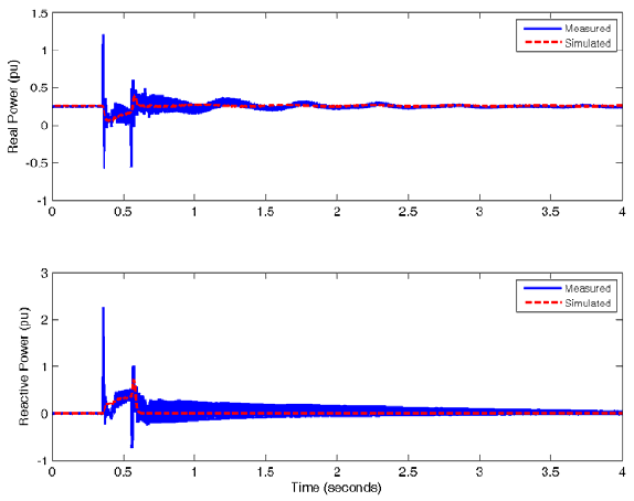
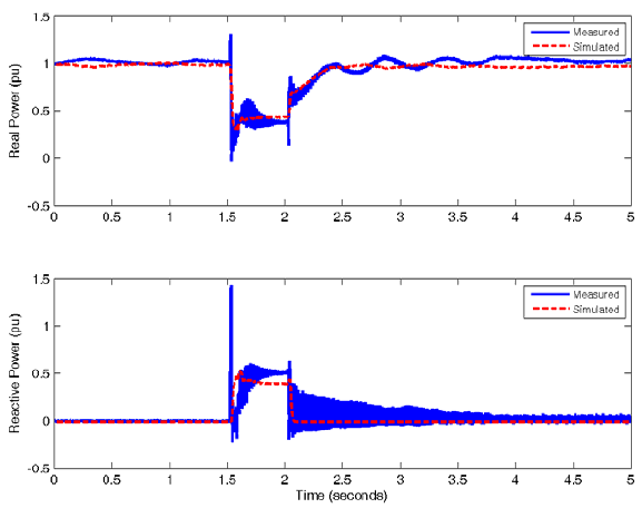
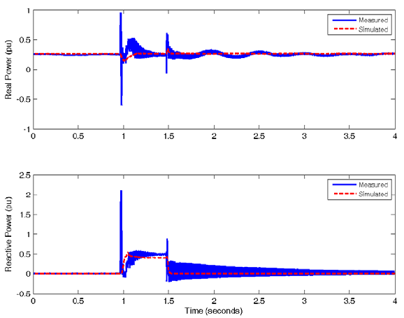
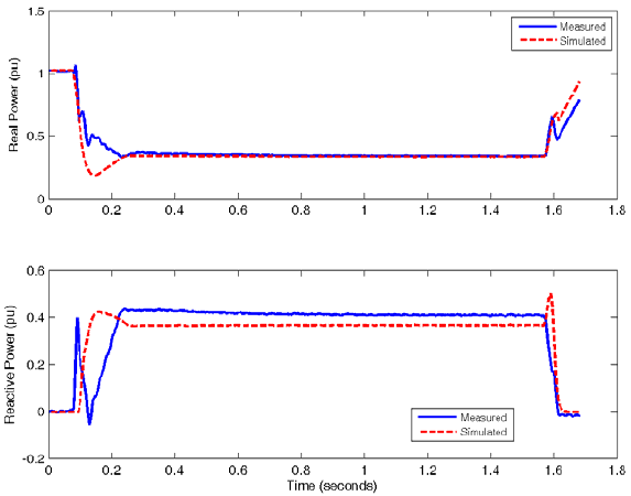
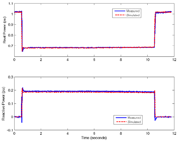
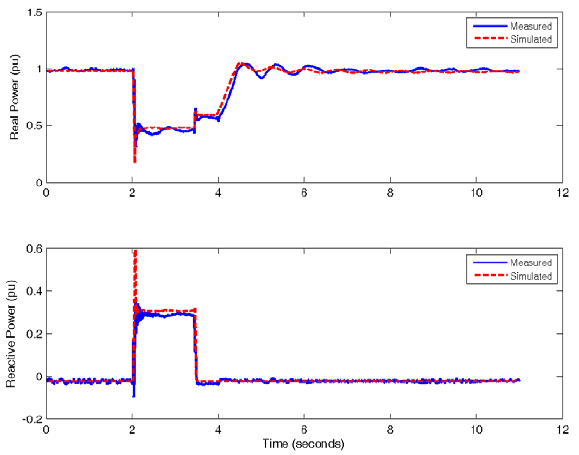
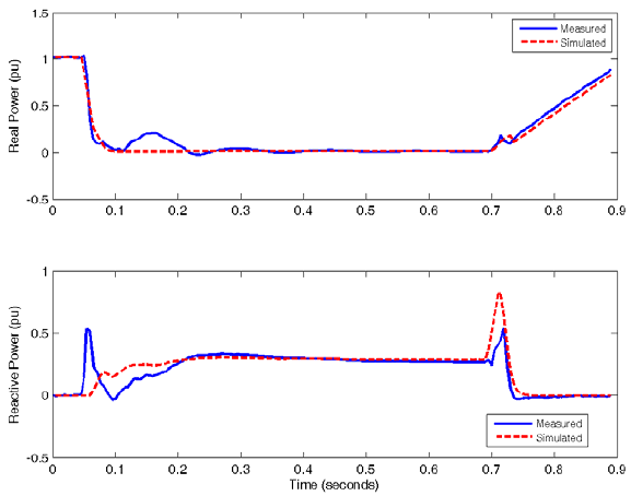
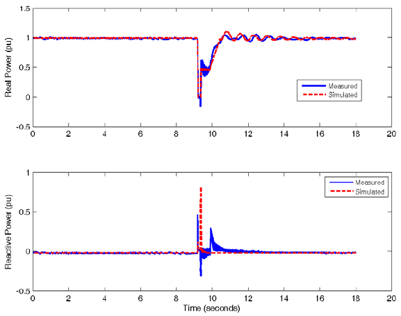
Here we present simulations using the newly proposed type 3 model and provide a comparison between simulation and measured turbine response.
The data used here was provided to EPRI under non-disclosure agreements (NDA) with the various turbine manufacturers for the purpose of research and investigation of the suitability of the various model structures being developed and proposed. These vendors graciously agreed to allow the public dissemination of the research results, as presented here and in the other references. The actual data, however, is covered under the NDA and cannot be disclosed.
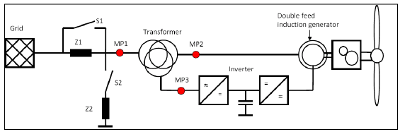
All the measured responses of WTGs shown here are for type 3 WTGs as measured on the lowvoltage side of the generator step-up transformer. That is, voltages and currents as measured on the low-voltage side of the generator transformer (points MP2 and MP3). In all the cases the real (P) and reactive (Q) power were calculated at point MP2 and MP3 using the three phase voltages and currents measured at those points, and then the total P and Q calculated by adding these quantities. Also, the voltage dips quoted here are as measured on the lowvoltage side of the generator transformer.
In the case of the measurements for the ABB unit, the data was measured for full factory tests of a doubly-fed asynchronous wind turbine generator while connected to the local utility grid through the generator step-up transformer. The unit was driven by a motor. In the case of the measurements for the Vestas units, the data was measured from a single doubly-fed asynchronous wind turbine generator in commercial operation inside a wind power plant, while connected to the power system. The following should be noted:
-
-
-
-
-
-
-
- The cases simulated for ABB – In general the fits look reasonable. The fits for voltage dips of 20% or so are extremely good. For the deeper voltage dips, since the active-crow bar circuit is engaged momentarily at the inception of the fault for purposes of protecting the power electronics, the initial transient in the real and reactive power are not emulated that well. This is because we have no representation of this control mechanism, or other similar controls used for protecting the power electronics during severe dips. The same set of model parameters were used to simulate all three events. Currently a proposal for capturing the behavior of the crow-bar is being discussed, however, at this stage the WECC REMTF decided not to pursue implementation of this proposal for the next release of the type 3 generic model.
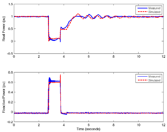
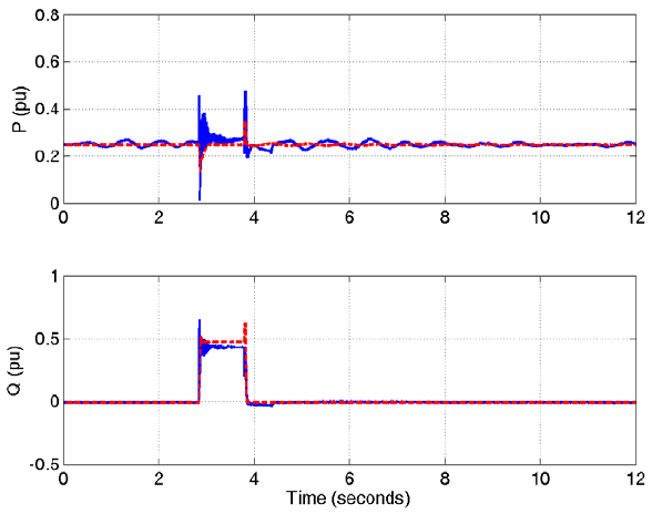
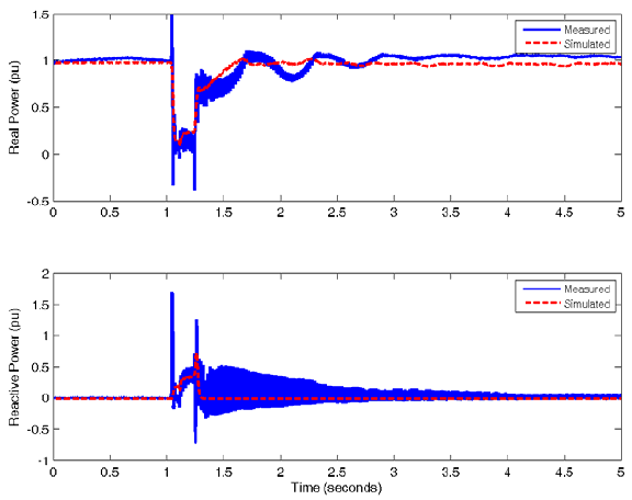
- The cases simulated for – Vestas – In general the fits look good. There are two sets of cases for two different designs of the type 3 machine. The fits for the reactive power response are quite good and we believe as good as the type 4 fits. There are several pertinent comments to be made:
- The oscillations in real power post fault do not match perfectly. The reason for this, we believe, is the simplicity of the generic models. There are two issues that we believe cannot be adequately modeled with the generic models. The damping of the torsional oscillation in the actual equipment is achieved by active damping controls and so is not a simple constant as modeled here. Secondly, the details of the electrical coupling of the machine to the grid, through the stator of the generator, and the details of the controls associated with the grid interaction are very much simplified. Currently a proposal for augmenting the model to allow for a simple representation of the active damping control is discussed to try to address one of these issues. However, at this stage the WECC REMTF decided not to pursue implementation of this proposal for the next release of the type 3 generic model.
- Another issue is that we can see (particularly Vestas 20-30% at full-load and 30-40% at full load) that there appears to be a delay from when the fault clears to when the real power starts to ramp back up to its pre-fault value. To emulate this behavior, we introduced a new parameter (Thld2) which is simply a time delay during which the maximum real current limit is kept at the value during the fault before it is released. This was set to 0.5 seconds in all cases.
- Finally, we noticed that for the Vestas case (30-40% at full-load) the gain on the reactive current injection during the fault (Kqv) seems to be different to the other cases. This was confirmed by Vestas – namely, for that particular test this value was apparently changed.
-
-
-
-
-
-
The user should realize that this model (as with any positive sequence models used in interconnected power system simulations) is a simplified model for the purpose of emulating the behavior of equipment for system wide planning studies. As such, for the most part the fitted model parameters do not necessarily directly correspond to actual equipment settings or physical quantities. In addition, further analysis was done on partial load conditions as well as another type 3 design for Vestas; some example simulations for these cases are also shown here.
All the cases presented here, are for balanced disturbances. For unbalanced conditions positive sequence models will likely not be suitable. This is particularly true for the type 3 machines. Such applications (i.e. for unbalanced faults) require further investigation.
Conversion Between The 1st and 2nd Generation Wind Turbine Generator Models
The following tables show how to convert the old (1st generation) generic stability models for type 3 WTGs to the new (2nd generation) models. The 1st generation models are a subset of the more general 2nd generation models, with a few exceptions:
- The older model did not have a current limit on the output; this is estimated based on the flux limit.
- The older model had the ability to bypass the second integrator in the reactive control path (i.e. set vltflg = 0 in the old model). This is not available in the new reec_a model, since at the time of developing the reec_a model the consensus was that this option is rarely if ever used.
- The new RES suite of models which were developed through a truly collaborative effort and so a single central model specification was developed; this meant that the new models are essentially identical among the commercial software platforms that have adopted them. Much effort was made to ensure a one to one correspondence in the parameter lists and to compare simulations across the platforms. This is not necessarily true of the older (1st generation) models. As such, the user will quickly notice significant differences between the implementation of the 1st generation models across some of the software platforms. We clearly cannot address these issues at this point in time, since we neither had an influence on the initial development of the older (1stgeneration) models, nor is it wise to try to address the differences now when those models are to be in time replaced by the newer models.
| New Model | Older Model |
|---|---|
| regc_a | wt3g |
| reec_a | wt3e (part of) |
| repc_a | wt3e (part of) |
| wtgp_a | wt3p |
| wtgt_a | wt3t (part of) |
| wtga_a | wt3t (part of) |
| wtgq_a | wt3e (part of) |
Therefore, with the above in mind, the conversion tables developed here are based on the GE (PSLF™) implementation of the 1st generation (older) generic models. The response of the converted model will not be exactly the same due to the differences explained above. In particular, if a two-mass shaft model is used Dshaft may have to be slightly modified in the 2nd generation model to yield the same level of damping.
It should also be noted that the new 2nd generation models were developed with the expressed intention of making them more flexible to allow modeling of a larger variety of equipment. With that in mind where older (1st generation) models exist in dynamic databases to represent existing equipment, they may not necessarily have been very representative of the equipment performance (specifically for none GE units); thus converting them through the conversion tables presented below will not yield a better representation of the units. In all cases the best approach is to consult the equipment vendor to come up with appropriate parameters for the 2nd generation models to represent the actual wind power plants (even in the case of GE units).
| New Model | Old Model | Explanatory Comments |
|---|---|---|
| regc_a | wt3g | Comments |
| Lvplsw | Lvplsw | |
| Rrpwr | Rrpwr | |
| Brkpt | Brkpt | |
| Zerox | Zerox | |
| Lvpl1 | Lvpl1 | |
| Vtmax | Volim | |
| Lvpnt1 | Lvpnt1 | |
| Lvpnt0 | Lvpnt0 | |
| qmin | Iolim | |
| accel | Khv | |
| Tg | Td | |
| Tfltr | Tfltr | |
| iqrmax | 999 | disable limit; no equivalent in old model |
| iqrmin | -999 | |
| Xe | Lpp | |
| wtgp_a | wt3p | Comments |
| Kiw | Kip | |
| Kpw | Kpp | |
| Kic | Kic | |
| Kpc | Kpc | |
| Kcc | 0 | disable; no equivalent in old model |
| Tpi | Tpi | |
| Pimax | Pimax | |
| Pimin | Pimin | |
| Piratmx | Pirat | |
| Piratmn | -Pirat | |
| wtgt_a | wt3t | Comments |
| Ht | Hfrac * H | |
| Hg | H – Ht | |
| Dshaft | Dshaft | In the wtgt_a model D does not exist; Dshaft may also need to be adjusted to get the same result as in the wt3t model |
| Kshaft | \(2\times\left(2\times\pi\times Freq1 \right)^2\times Ht \times \left(\frac{Hg}{H} \right)\) | |
| wo | 1 | this value will be set to ωref upon initialization by the wtgq_a modelwtga |
| wtga_a | wt3t | Comments |
| Ka | Kaero | |
| Theta0 | 0 | set to default; no equivalent in old model |
| wtgq_a | wt3e | Comments |
| Kip | Kitrq | |
| Kpp | Kptrq | |
| Tp | 0 | not available in old model so disable |
| Twref | Tsp | |
| Temax | Pmax/Wp100 | |
| Temin | Pmin/Wpmin | |
| p1 | Pmin | |
| spd1 | Wpmin | |
| p2 | 0.2 | |
| spd2 | Wp20 | |
| p3 | 0.6 | |
| spd3 | Wp60 | |
| p4 | Pwp100 | |
| spd4 | Wp100 | |
| Tflag | 0 | not available in old model so disable |
| reec_a | wt3e | Comments |
| vdip | 0 | not available in old model so disable |
| vup | 2 | |
| Trv | Tr | |
| dbd1 | -1 | not available in old model so disable |
| dbd2 | 1 | |
| kqv | 0 | |
| iqh1 | 0.001 | |
| iql1 | -0.001 | |
| vref0 | 1 | |
| iqfrz | 0 | |
| thld | 0 | |
| thld2 | 0 | |
| Tp | Tp | |
| Qmax | Qmax | |
| Qmin | Qmin | |
| Vmax | Vmax | |
| Vmin | Vmin | |
| kqp | 0 | not available in old model so disable |
| kqi | Kqi | |
| kvp | 0 | not available in old model so disable |
| kvi | Kqv | |
| vref1 | 0 | not available in old model so disable |
| tiq | 0.02 | set to default value |
| dpmax | Pwrat | |
| dpmin | -Pwrat | |
| Pmax | Pmax | |
| Pmin | Pmin | |
| imax | Xiqmax/Lpp | wt3e had no current limit so set to estimated current limit based on flux limit; Lpp comes from wt3g model |
| Tpord | Tpc | |
| pfflag | 1 if varflg = -1 or 0 if varflg = 0 or 1 | |
| vflag | 1 | set to 1 since no equivalent in old model |
| qflag | 1 if vltflg = 1 | for the case that vltflg = 0 in the old model, this option is not available in the new models; this was rarely used |
| pflag | 0 | must be set to 0 for the implementation in GE PSLF® |
| pqflag | 1 | set to 1 since no equivalent in old model |
| vq1 | 0 | not available in old model so set to constant value across all voltages |
| iq1 | Xiqmax | |
| vq2 | 0.1 | |
| iq2 | Xiqmax | |
| vq3 | 0.9 | |
| iq3 | Xiqmax | |
| vq4 | 1 | |
| iq4 | Xiqmax | |
| vp1 | 0 | |
| ip1 | ipmax | |
| vp2 | 0.1 | |
| ip2 | ipmax | |
| vp3 | 0.9 | |
| ip3 | ipmax | |
| vp4 | 1 | |
| ip4 | ipmax | |
| repc_a | wt3e | Comments |
| Tfltr | Tr | |
| Kp | Kpv | |
| Ki | Kiv | |
| Tft | 0 | not available in old model so disable |
| Tfv | Tc | |
| refflg | 1 | not available in old model so disable |
| vfrz | 0 | |
| rc | 0 | |
| xc | Xc | |
| Kc | 0 | |
| vcmpflg | 1 | the branch for monitoring the voltage is set differently in various software platforms; check the software user’s manual |
| emax | 99 | not available in old model so disable |
| emin | -99 | |
| dbd | 0 | |
| Qmax | Qmax | |
| Qmin | Qmin | |
| kpg | 0 | not available in old model so disable |
| kig | 0 | |
| Tp | Tp | |
| fdbd1 | 0 | not available in old model so disable |
| fdbd2 | 0 | |
| femax | 0 | |
| femin | 0 | |
| pmax | Pmax | |
| pmin | Pmin | |
| tlag | 0 | |
| ddn | 0 | |
| dup | 0 | |
| frqflg | 0 | |
| outflag | 0 |
Conclusion and Summary
At this point, with the gracious input of the various equipment vendors for type 3 wind turbine generators, a proposed model is on the table that appears to cater to at least three designs tested so far.
A key feature of the proposed type 3 model is that it is modularized. That is, it is made of seven modules several of which are identical to the type 4 model.
All the cases presented here are for balanced disturbances. For unbalanced conditions positive sequence models will likely not be suitable. This is particularly true for the type 3 machines. This requires further investigation.
Finally, it should be kept in mind that the model under discussion here is a “generic” model for interconnected power system stability simulations and so one needs to keep the models simple, while catering to as wide a possible range of equipment. It would be an insurmountable task to try to achieve a model that would cater to every possible equipment configuration. Therefore, when doing detailed plant specific studies, vendor specific models (obtained directly from the equipment vendors) will still always be the best option. The “generic” models are for bulk system studies performed by TSOs, TOs, reliability entities, etc.
References
- ↑ WECC REMTF, “Specification of the Second Generation Generic Models for Wind Turbine Generators ”, Prepared under Subcontract No. NFT-1-11342-01 with NREL (last revised 11/11/13). [Online]. Available: https://www.wecc.biz/Reliability/WECC-Second-Generation-Wind-Turbine-Models-012314.pdf [Accessed June 2015].
- ↑ EPRI, “Proposed Changes to the WECC WT3 Generic Model for Type 3 Wind Turbine Generators”, Prepared under Subcontract No. NFT-1-11342-01 with NREL, Issued to WECC REMTF and IEC TC88 WG27 03/26/12 (revised 6/11/12, 7/3/12, 8/16/12, 8/17/12, 8/29/12, 1/15/13, 1/23/13, 9/27/13).
- ↑ Generic Models and Model Validation for Wind and Solar PV Generation: Technical Update. EPRI, Palo Alto, CA: 2011, 1021763. [Online]. Available:http://www.epri.com/abstracts/pages/productabstract.aspx?ProductID=000000000001021763
- ↑ Model User Guide for Generic Renewable Energy System Models:Technical Update, June 2015, 3002006525. [Online]. Available:http://www.epri.com/abstracts/Pages/ProductAbstract.aspx?ProductId=000000003002006525
- ↑ 5.0 5.1 Siemens Energy, Inc., PSSE Wind Model Library, Schenectady, NY, 2009.
- ↑ 6.0 6.1 GE Energy, PSLF Version 17.0_07 User’s Manual, Schenectady, NY, 2010.
- ↑ Nicholas W. Miller, Juan J. Sanchez-Gasca, William W. Price, Robert W. Delmerico, “Dynamic Modeling of GE 1.5 and 3.6 MW Wind Turbine-Generators for Stability Simulations”, Proc. Power Engineering Society General Meeting 2003. Toronto, Ontario. July 2003.
- ↑ K. Clark, N. W. Miller, J. J. Sanchez-Gasca, Modeling of GE Wind Turbine-Generators for Grid Studies, Version 4.5, April 2010, General Electric International, Inc.
- ↑ Thomas Ackermann, Wind Power in Power Systems, 2nd Edition, Wiley, May 2012 (ISBN: 978-0-470-97416-2)
- ↑ J. Fortmann, S. Engelhardt, J. Kretschmann, C. Feltes and I. Erlich, “Validation of an RMS DFIG Simulation Model According to New German Model Validation Standard FGW TR4 at Balanced and Unbalanced Grid Faults”, 8th International Workshop on Large-Scale Integration of Wind Power into Power Systems as well as on Transmission Networks for Offshore Wind Farms, Bremen, Germany, 2009.