
Author: Sandia National Laboratories[1]
We report an uncertainty and sensitivity analysis for modeling DC energy from photovoltaic systems. We consider two systems, each comprised of a single module using either crystalline silicon or CdTe cells, and located either at Albuquerque, NM, or Golden, CO. Output from a PV system is predicted by a sequence of models. Uncertainty in the output of each model is quantified by empirical distributions of each model’s residuals. We sample these distributions to propagate uncertainty through the sequence of models to obtain an empirical distribution for each PV system’s output. We considered models that: (1) translate measured global horizontal, direct and global diffuse irradiance to plane-of-array irradiance; (2) estimate effective irradiance from plane-of-array irradiance; (3) predict celltemperature; and (4) estimate DC voltage, current and power.
We found that the uncertainty in PV system output to be relatively small, on the order of 1% for daily energy. Four alternative models were considered for the POAirradiance modeling step; we did not find the choice of one of these models to be of great significance. However, we observed that the POA irradiance model introduced a bias of upwards of 5% of daily energy which translates directly to a systematic difference in predicted energy. Sensitivity analyses relate uncertainty in the PV system output to uncertainty arising from each model. We found that the residuals arising from the POA irradiance and the effective irradiance models to be the dominant contributors to residuals for daily energy, for either technology or location considered. This analysis indicates that efforts to reduce the uncertainty in PV system output should focus on improvements to the POA and effective irradiance models.
Contents
Introduction
As the photovoltaic (PV) industry continues to mature and incentives are reduced, investment in PV increasingly depends on the confidence that can be placed in predictions of the energy yield. Predicting energy yield requires use of a sequence of models, e.g., to translate measured irradiance to the system’s plane-of-array, to estimate cell temperature, and to predict DC power for given conditions. Uncertainty in these models and their inputs arises from a variety of sources, including measurement errors, inexact model specification, and from the necessarily finite data used to calibrate models. In aggregate, these uncertainties contribute to uncertainty in predicted energy yield. Therefore, to understand what confidence can be placed in energy yield predictions, to identify how to improve model accuracy and to reduce prediction uncertainty, we must quantify the uncertainty introduced by each model and the effect of each model’s uncertainty on energy yield predictions.
Previous analyses of uncertainty in module or system performance has centered on measurement uncertainties of outdoor installations, or on calibration of models to data assumed to be exact. For example, a detailed investigation of module performance uncertainties under natural sunlight including correction for irradiance and temperature was given by Whitfield et al.[2]. The methodology was based on the analytical propagation of respective uncertainties in two dimensions using the Guide to the Expression of Uncertainty in Measurement (GUM). This methodology was used and expanded for long-term outdoor IV measurements for data of Northern latitude.[3] The Parameter Uncertainty paper examined the influence of uncertainty in calibrated parameters on performance predictions, where the data used for calibration was assumed to be error-free.
Methodology
Conceptual Approach to Uncertainty Analysis
Uncertainty analysis is a systematic process to propagate uncertainty in a model or its inputs to uncertainty in the model’s output. An uncertainty analysis involves two primary steps: quantification and propagation. First, we quantify uncertainty in a model and in the model’s inputs. Here we use probability distributions to quantify uncertainty, noting that other expressions of uncertainty are available[4]. Second, we propagate uncertainty to a model’s output through a set of model calculations using a Monte Carlo technique to sample distributions for uncertainty.
In concept, uncertainty can be categorized as either parameter uncertainty or model uncertainty. Parameter uncertainty refers to uncertainty in a particular model input, whereas model uncertainty refers to lack of knowledge regarding the model itself. In practice, these two categories tend to overlap, for example, a model for extraterrestrial irradiance may consist of a single, constant (but uncertain) value, or may comprise an equation involving several parameters that accounts for observed systematic variation in extraterrestrial irradiance over time.
In our analysis, we explicitly address model uncertainty by considering several credible alternative models, when such models are available. However, we do not represent parameter uncertainty in the traditional manner, which would be to specify a distribution of possible values for each individual parameter. Instead, we adopt an approach where we characterize the uncertainty in a model’s output by quantifying the distribution of each model’s residual, i.e., the difference between the model’s prediction and the true value. This method of representing uncertainty in a model’s residuals effectively aggregates the uncertainty resulting from all of the model’s parameters into a single quantity.
We adopt this approach because nearly all models involved in estimating PV system output are calibrated, i.e., their parameter values are determined by fitting the model’s equations to data that are considered representative. When a parameter is determined by fitting an equation to a set of data, uncertainty in the parameter arises from a number of sources, including uncertainty in the data used for the fitting, model uncertainty in the equation used, and numerical error arising from the finite sample of data and the fitting procedure. Moreover, when the parameter is jointly determined with other parameters, uncertainty in each parameter is likely correlated with uncertainty in all other parameters determined in the same fitting procedure. These factors complicate the effort to separately describe uncertainty in each fitted parameter.
PV System Modeling

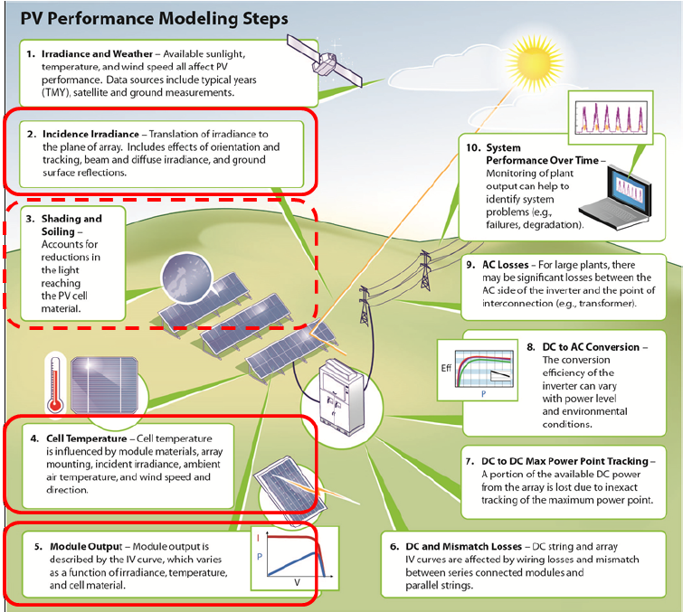
The process of modeling DC power output from a PV system involves nine notional steps, as illustrated in the PV System Modeling Process figure. Uncertainty in the outcome of each step may arise from uncertainty in the models employed or from the parameters required by those models. For example, Step 2, Incident Irradiance, estimates plane-of-array (POA) irradiance from measured irradiance (GHI, DNI and/or DHI). This translation involves choice among a number of models for sky diffuse irradiance, e.g., the isotropic sky diffuse model or Hay and Davies’ diffuse model[5].
The Sequence of Models Considered figure indicates the sequence of models considered in the quantification of uncertainty for PV system modeling. Not all modeling steps shown in the PV System Modeling Process figure are addressed in the uncertainty quantification illustrated by the Sequence of Models Considered figure. We intentionally did not consider uncertainty represented by the models and measurements in Step 1, because that uncertainty is dominated by uncertainty in measured irradiance which will directly (and proportionally) affect predicted power. There are several ongoing research programs to better understand and improve measurement uncertainty. Our focus is to understand the relative contribution of all other modeling steps.
To quantify uncertainty in the outcome of any particular modeling step, we needed concurrent measurements of model inputs and outputs with sufficient resolution and/or quality to have confidence that the data would fairly represent the uncertainty present. We found data only for those steps indicated by the Sequence of Models Considered figure. For Step 3, we found data only for the part of this step that addresses the effects of varying solar spectrum on module output, termed spectral mismatch, but nor for the other aspects of Step 3, which concern surface reflection losses, shading and soiling.
We define a total of four scenarios: two locations (Albuquerque, NM and Golden, CO) and two modules (a SunPower 305WHT and a FirstSolar 272). In each scenario we consider a single PV module at fixed latitude tilt. We use GHI, DNI and DHI measured during 2011 at each location. All models illustrated in the Sequence of Models Considered figure except the plane-of-array irradiance models require modulespecific coefficients, which we determine from measurements made in Albuquerque, NM. Assuming specific locations reduces somewhat the generality of our study’s conclusions, because model calibration and model residuals are determined from site-specific data. However, as we will describe, our analysis focuses on the relative influence of various uncertainties on the uncertainty in the modeling outcomes, rather than on the absolute values of the modeling outcomes. We do not believe that our use of site-specific data greatly affects our study’s conclusions.
Methods for Uncertainty Quantification
Let \(\hat{f}\left (x\mid p \right)\) represent a model \(\hat{f}\) applied to inputs x with a fixed set of parameter values p. Denote the true value at x by \(f(x)\); then the residual is given by:
\(\epsilon_f\left (x\mid p \right) = \hat{f}\left (x\mid p \right)-f\left (x \right)\)We regard \(\epsilon_f\left (x\mid p \right)\) as a random variable and develop distributions for \(\epsilon_f\left (x\mid p \right)\) for each selected model \(\hat{f}\) using the representative data.
The distribution for \(\epsilon_f\left (x\mid p \right)\) characterizes the aggregate uncertainty in the model \(\hat{f}\) and the inputs x conditional on the parameters p. Different distributions for \(\epsilon_f\left (x\mid p \right)\) can result when the parameters p are varied. Because parameters are generally obtained by calibration of a model to data, for a given set of data there is a best value for these parameters, but other values may arise from different data sets. Thus parameter variation can arise from alternate data sets, which in turn results if the analysis is done using measurements from a different location or time of year.
Parameter values used here are those regarded as default values for each model. We did not attempt to quantify uncertainty in the parameters by finding alternate data sources and recalibrating models to obtain alternate parameter values.
As indicated in the Sequence of Models Considered figure, calculation of DC power from a PV system involves a sequence of models. At each step in the process, uncertainty is quantified for the models used in that step. Results (with uncertainty) from each step are then used as input to the next step.
Step 1: Estimation of POA irradiance
Plane-of-array (POA) irradiance GPOA is defined as the total broadband irradiance incident on the face of a module. We estimate POA irradiance using a model \(\hat{f}_{POA}\) that operates on GHI, DNI and DHI:
\(\hat{G}_{POA}(t) = \hat{f}_{POA} \left (GHI(t), DNI(t), DHI(t)\mid p_{POA} \right)\)We consider the following models for \(\hat{f}_{POA}\): isotropic sky diffuse; Sandia simple sky diffuse, Hay and Davies; and Perez. Expressions for \(\hat{f}_{POA}\) can be complex and are found in the listed references, along with each model’s parameter values.
For POA irradiance models, the residual \(\delta_{POA}\left (t\mid p_{POA} \right)\) is expressed a fraction of the measured POA, denoted by POA(t):
We expressed the residual as a fraction because it allowed for a simpler detrending of the residuals as functions of the solar angle of incidence (AOI) (see here for details). Measured GHI, DNI, DHI and POA were obtained for 2011 at Sandia National Laboratories in Albuquerque, NM, and from NREL’s Solar Radiation Research Laboratory in Golden CO. At Sandia, GHI is measured with Kipp and Zonen CMP11 pyranometer, and DHI and POA irradiance are measured with Eppley PSPpyranometer. DNI is measured with a CHP-1 pyrheliometer. At NREL GHi and DHI are measured with Kipp and Zonen CM22 pyranometers, DNI is measured with a Kipp and Zonen pyheliometer, and POA irradiance is measured with a Eppley PSP pyranometer tilted at 40° to the south.
Analysis of POA residuals revealed systematic trends in \(\delta_{POA}\left (t\mid p_{POA} \right)\) that changed with time of day, season, location and POA model (see here). To facilitate random sampling from these results, we fit empirical expressions \(\gamma_{POA} \left (t\mid p_{POA} \right)\) to the residuals to separate trends from random effects:
\(\delta_{POA}\left (t\mid p_{POA} \right) = \gamma_{POA} \left (t\mid p_{POA} \right)+\epsilon_{POA} \left (t\mid p_{POA} \right)\)Illustrative results are provided here for each POA model.
Step 2: Estimation of effective irradiance
Effective irradiance E represents the irradiance converted to electrical power within the module. E is reduced from POA by: reflection losses at the module’s face; the module’s quantum efficiency, commonly expressed as a modifier representing change in current with changes in spectrum; and parasitic losses from resistances internal to the module. Models are available to separately quantify reflection and spectral losses. Parasitic losses are normally accounted for by the module performance model (see Step 4). We do not consider reflection or parasitic losses in our analysis, because we did not find sufficient data to quantify residuals in these models. The effective irradiance is modeled using a common empirical expression:
\(\begin{align}\hat{E}\left (t\mid p_E \right) & = \hat{f}_E\left (AM(t)\mid p_E \right)\hat{G}_{POA}(t)\\
& = \left [p_{E,4}AM(t)^4+p_{E,3}AM(t)^3+p_{E,2}AM(t)^2+p_{E,1}AM(t)+p_{E,0}\right ]\hat{G}_{POA}(t)\\
\end{align}\)
where AM is the absolute air mass calculated from the solar position and site altitude, using tools coded in the PV_Lib toolbox. The parameter vector pE is determined by fitting the expression in equation above to measured module short-circuit current. Solar position (i.e., zenith Z (degrees) and azimuth Az (degrees)) was computed using legacy algorithm originating with G. Hughes[6]. Relative air mass AMr is calculated using the empirical model described in Kasten and Young[7]:
\(AMr = \cfrac{1}{cos(Z)+0.50572\times \left (6.07995+(90-Z)\right )^{-1.6364}}\)Site pressure P (Pa) was estimated from site elevation H (m)
\(P = 100\times \left (\cfrac{44331.514-H}{11880.516}\right )^{1/0.1902632}\)and absolute air mass AM is obtained as:
\(AM = AMr\times \cfrac{P}{101325}\)No uncertainty is ascribed to the models represented by the calculations in the three equations above.
Effective irradiance is not measured directly. Rather, effective irradiance is calculated from measured short-circuit current ISC and cell temperature TC:
\(E = \cfrac{I_{SC}}{I_{SC0}\left (1+\alpha_{I_{SC}}(T_C-25)\right )}\)ISC0 is the pre-determined value for ISC at standard test conditions (STC; 1000 W/m2 and 25°C) and αIsc is the pre-determined value for the temperature coefficient of ISC. These values were estimated from testing of each module at Sandia National Laboratories using Parameter Uncertainty techniques. Cell temperature TC is calculated from measured short-circuit current and open-circuit voltage using a technique similar to IEC 60904-5:2011.
The residual for effective irradiance is quantified by the difference between modeled values \(\hat{E}\left (t\mid p_E \right )\) and values E(t) calculated from measurements:
\(\epsilon_E\left (t\mid p_E \right ) = \hat{E}\left (t\mid p_E \right )-E(t)\)Illustrative results for the residuals are shown here.
Step 3: Estimation of cell temperature
We model cell temperature TC(t) using the empirical approach proposed by Sandia Array Performance Model
\(\begin{align}\hat{T}_C(t) & = \hat{f}_{TC}\left (\hat{G}_{POA}(t),Tamb(t),WS(t)\mid P_{TC}\right )\\
& = \hat{G}_{POA}(t)exp\left (a+bWS(t)\right )+Tamb(t)+\cfrac{\hat{G}_{POA}(t)}{1000~W/m^2}\Delta T\\
\end{align}\)
where Tamb(t) is ambient air temperature and WS(t) is the wind speed. The parameter vector pTC=(a,b,ΔT) is determined by fitting the expression in equation above to module temperatures measured over a range of irradiance, air temperature and wind conditions.
Cell temperature TC is not measured directly. Rather, TC is calculated from measured shortcircuit current and open-circuit voltage using a technique similar to IEC 60904-5:2011. The residual for cell temperature is quantified by the difference between modeled values \(\hat{T}_C\left (t\right )\) and values TC(t) calculated from measurements:
Illustrative results are provided in here.
Step 4: Calculation of DC power
We obtain DC power PDC(t) by separately predicting DC voltage VDC(t) and current IDC(t) from the PV modules by using the Sandia Array Performance Model (SAPM) \(\hat{f}_{DC}\)
\(\left [\hat{V}_{DC}\left (t\mid p_{DC} \right ),\hat{I}_{DC}\left (t\mid p_{DC} \right )\right ] = \hat{f}_{DC}\left (\hat{E}(t),\hat{T}_C(t)\mid p_{DC} \right)+\left [\epsilon_{VDC}\left (t\mid p_{DC} \right ),\epsilon_{IDC}\left (t\mid p_{DC} \right )\right ]\)In the above equation the residuals
\(\epsilon_{VDC}\left (t\mid p_{DC} \right )\)and
\(\epsilon_{IDC}\left (t\mid p_{DC} \right )\)represent the residuals for DC voltage
\(\hat{V}_{DC}\left (t\right )\)and current
\(\hat{I}_{DC}\left (t\right )\), respectively. DC power (with uncertainty) is then determined by multiplying:
\(\hat{P}_{DC}\left (t\mid p_{DC} \right ) = \hat{V}_{DC}\left (t\mid p_{DC} \right )\times \hat{I}_{DC}\left (t\mid p_{DC} \right )\)The parameter vector pDC contains 13 module-specific values that are determined from measurements of module output during a sequence of performance tests. The residuals
\(\epsilon_{VDC}\left (t\mid p_{DC} \right )\)and
\(\epsilon_{IDC}\left (t\mid p_{DC} \right )\)are quantified by comparing modeled values with measured IV curves. Illustrative results are provided here.
Quantifying Uncertainty
We describe the quantification of uncertainty for each modeling step: POA irradiance; effective irradiance; cell temperature; and DC power.
POA Irradiance

.png)
![]()
.png)
![]()

![]()
.png)
Estimating POA irradiance from GHI, DNI and DHI requires estimating the beam and diffuse components, respectively Eb and Ediff:
Beam irradiance Eb is determined from DNI by accounting for the sun’s angle of incidence AOI on the module:
\(E_b = DNI\times cos\left (AOI\right)\)Angle of incidence AOI is computed using the module’s assumed fixed orientation (latitude tilt and 180° azimuth) and the sun position computed using legacy algorithm originating with G. Hughes, which has sufficiently high accuracy that we did not consider uncertainty in AOI.
The diffuse component is divided into ground reflected irradiance Ediff,g and sky diffuse irradiance Ediff,sky:
Ground reflected irradiance Ediff,g is estimated using an uncertain value for ground albedo a:
\(E_{diff,g} = GHI\times a\times \cfrac{1-cos\left (A\right)}{2}\)where A is the tilt angle of the module towards the equator (assumed constant and precisely known). The model for Ediff,g in the above equation assumes horizontal surrounding terrain and isotropic reflection of GHI from the ground that is independent of solar zenith angle, solar azimuth, or time of day. Thus, the albedo parameter a represents a spatially and temporally averaged fraction of GHIreflected from the ground. No precise quantification of albedo is available. It is typical to assume a value a = 0.2.[8] We use 0.2 as a base value and test whether our analysis depends on this value (seesee here).
Sky diffuse irradiance Ediff,sky is calculated using one of four alternative models (listed in order of increasing model complexity):
- Isotropic sky diffuse model;
- Sandia simple sky diffuse model;
- Hay and Davies diffuse model[5];
- Perez sky diffuse model.
For models that require parameter values we used values generally regarded as typical, as follows:
- Sandia simple sky diffuse model – empirical coefficients 0.12 and 0.004. These values were determined by calibrating the model to measurements of GHI, DHI, and ambient temperature prior to 2010.
- Hay and Davies diffuse model – annual average extraterrestrial radiation Ea taken equal to 1367 W/m2.
- Perez sky diffuse model – the Perez model requires a large number of empirical coefficients. We used values that are regarded as typical and recommended by the model’s originators.
For each model we determined an empirical distribution for the model residuals using concurrent measurements of GHI, DNI, DHI and POA irradiance at Sandia’s Photovoltaic Systems Evaluation Laboratory during 2011. We used measured GHI, DNI and DHI to predict POA irradiance then computed model residuals by comparing predicted to measured POAirradiance. Using scatterplots and other techniques, we identified systematic trends in the residuals that are reflected in the characterization of uncertainty in each model’s residuals.
To avoid including residuals primarily resulting from measurement artifacts we exclude data measured with sun elevation angles less than 10°. At the PSEL site, local shadowing occasionally affects measurements at low sun elevation angles. In addition, the instrument used to measured POA irradiance (an Eppley PSP pyranometer) shows measurement aberrations due to internal reflections at high incident angles. For these reasons our analysis precludes low sun elevation angles.
Isotropic Sky Diffuse Model
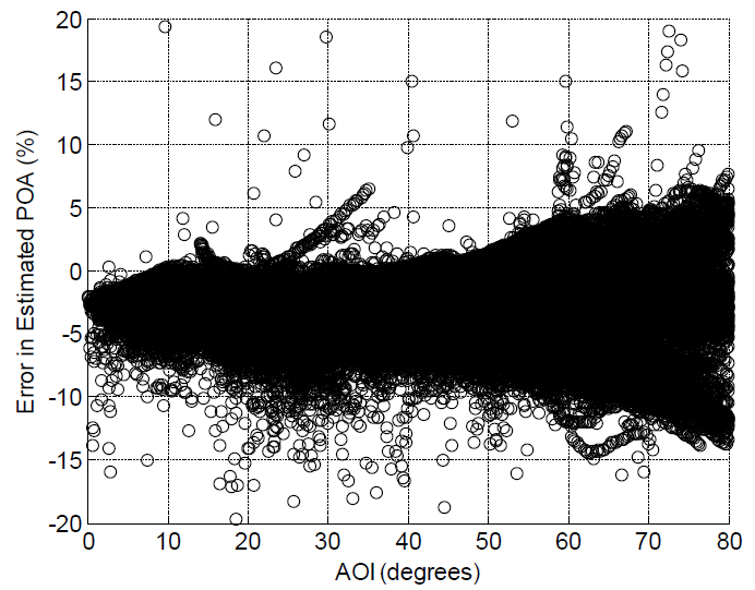
The Dependence on sky condition figure displays the residuals for the Isotropic sky diffuse model as a function of angle of incidence AOI . Dependence of the residuals on AOI is evident. The Dependence on time of year figure shows residuals for two different months and demonstrates dependence of residuals on time of year. The Dependence on sky condition figure illustrates that residuals are different for clear sky conditions as opposed to cloudy conditions. Finally, the Dependence on time of day (clear periods) and Dependence on time of day (cloudy periods) figures show that residuals can also depend on time of day. In these figures, we separate residuals into two subsets (before and after noon), and fit each subset with a second order polynomial in AOI to quantify the different trends.
Accordingly, we assembled 48 empirical distributions for model residuals for the Isotropic clear sky model. For each month, we distinguished clear and cloudy conditions by the ratio between measured DHI and GHI: if the ratio was less than 0.2, we considered the sky to be clear. We further separate each day into am and pm time periods, to partition data for 2011 into 48 sets. Within each set we quantified the systematic dependence of the residuals on AOI by fitting a second order polynomial (as illustrated in the Dependence on time of day (clear periods) and Dependence on time of day (cloudy periods) figures). The polynomial fit is generally successful at removing the systematic trends (e.g., the Residuals for clear sky conditions and Residuals for cloudy conditions figures). We then estimated one (or more) empirical cumulative distribution functions (CDFs) from the difference between each residual and the fitted polynomial (e.g., the Empirical CDFs (clear sky conditions) and Empirical CDFs (cloudy sky conditions) figures). When the detrended residuals showed changes in variance across AOI, we partitioned AOI into several bins and obtained separate CDFs for each bin.
We note that the de-trended residuals exhibit a relatively consistent daily pattern during clear sky conditions but a rather random pattern during cloudy conditions. Accordingly, to propagate uncertainty we sample one quantile value for clear conditions for each day, but randomly sample a quantile value for each time for cloudy conditions.
Sandia Simple Sky Diffuse Model
.png)
For the Sandia simple sky diffuse model we adopted the same general approach for quantifying uncertainty in model residuals as is used for the Isotropic sky diffuse model. We observed a range of residuals generally comparable to the Isotropic sky diffuse model.
Hay and Davies Diffuse Model
.png)
For the Hay and Davies diffuse model we adopted the same general approach for quantifying uncertainty in model residuals as is used for the Isotropic sky diffuse model, and observed similar ranges of residuals.
Perez Sky Diffuse Model
.png)
.png)
For the Perez sky diffuse model we adopted the same general approach for quantifying uncertainty in model residuals as is used for the Isotropic sky diffuse model. Similar ranges of residuals are observed in these models.
Finally, comparing the various POA irradiance models, we observed that the systematic trends in model residuals are similar among the models, generally increasing from a negative value to a positive value as angle-of-incidence increases. Systematic trends in the residuals vary more by month of year for the isotropic sky and Sandia models, than for the Hay and Davies and Perez models, although the range of residuals is similar among all models.
Effective Irradiance
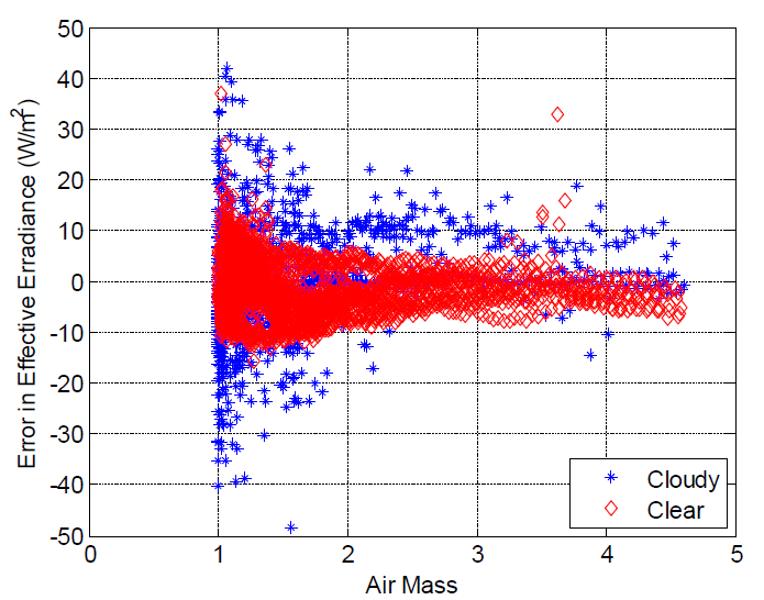
We determined an empirical distribution for the effective irradiance model’s residual using the measurements of POA irradiance and calculated air mass AM at Sandia’s PSEL during the days from March 7 through March 20, 2012, along with IV curves recorded during this same time period. We calculated effective irradiance using the measured IV curves as described in Step 2 of PV System Modeling chapter. We examined the residuals and found different behavior for different sky condition and ranges of air mass AM. Each time was characterized as clear or cloudy based on the ratio between measured DHI and GHI, where if the ratio was less than 0.2 that time was considered to be clear sky, while all others were considered cloudy. Conditional on clear or cloudy conditions, we then constructed a total of six distribution models for the residual in effective irradiance by partitioning air mass into three intervals:
\(\begin{align}Clear: & E1 = {0 < AM <1.2}\\
& E2 = {1.2 ≤ AM < 2}\\
& E3 = {2 ≤ AM}\\
\end{align}\) \(\begin{align}
Cloudy: & E4 = {0 < AM <1.2}\\
& E5 = {1.2 ≤ AM < 2}\\
& E5 = {2 ≤ AM}\\
\end{align}\)
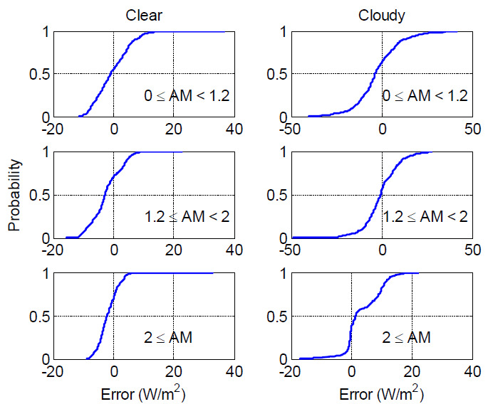
For each interval, we constructed an empirical distribution for the residuals. CDFs for the distributions are shown in the CDFs for Effective Irradiance Model Residual figure. Because the partitions for the distributions are not based on POA irradiance, the same distributions for effective irradiance are used with each of the four different POA irradiance models. Also, because calculated effective irradiance was obtained from the same measurements as were used to estimate the effective irradiance model in equation (5), the CDFs for residuals for effective irradiance are generally unbiased.
Cell Temperature


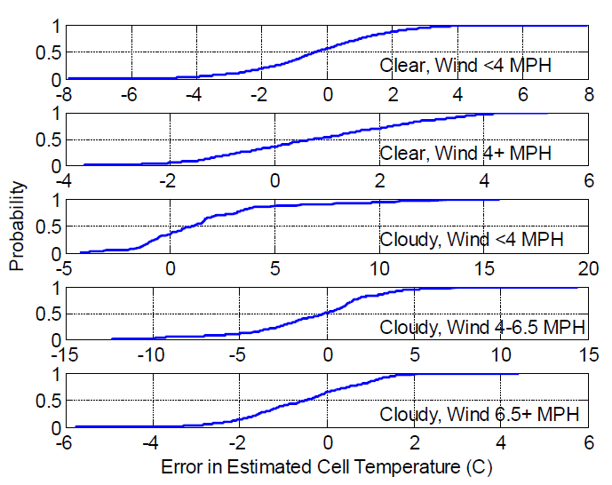
Cell temperature is modeled using equation (11). We determined an empirical distribution of the model residuals using measurements of POA irradiance, wind speed and ambient temperature at Sandia’s Photovoltaic Systems Evaluation Laboratory (PSEL) during the days from March 7 through March 20 2012, along with IV curves recorded during this same time. We estimated cell temperature from the IV curves using a technique similar to IEC 60904-5:2011, and computed a set of residuals by comparing modeled and estimated cell temperatures. We examined the residuals and found different behavior for different sky condition and ranges of wind speed WS. We created 5 empirical distributions for the model residuals. Each time was characterized as clear or cloudy based on the ratio between measured DHI and GHI, where if the ratio was less than 0.2 that time was considered to be clear sky, while all others were considered cloudy. Conditional on clear or cloudy conditions, we then constructed a total of five distribution models for the residual in cell temperature by partitioning wind speed into three intervals for cloudy periods and two for clear times:
Cloudy: & E1 = {0 < WS < 4}\\
& E2 = {4 < WS < 6.5}\\
& E3 = {6.5 < WS}\\
\end{align}\) \(\begin{align}
Clear: & E4 = {0 < WS < 4}\\
& E5 = {4 < WS}\\
\end{align}\)
For each interval an empirical CDF for the residuals in cell temperate was constructed. CDFs for the distributions are displayed in the Empirical CDFs for Cell Temperature Model Residual figure. Because the partitions for the distributions are not based on POA irradiance, the same distributions are used for each of the four POA models created above.
PV Module Output
The DC power and DC voltage figure shows measured DC power and DC voltage from testing of a SunPower 305-WHT crystalline silicon module at PSEL during September, 2009. Coefficients for the Sandia Array Performance Model (SAPM) are determined from these measurements. Model predictions of DC power and DC voltage are also displayed in the DC power and DC voltage figure.
We found that residuals in predicted DC current and predicted DC voltage to be uncorrelated (correlation coefficient 0.0067). We see a relatively strong correlation between effective irradiance and cell temperature, as should be expected.
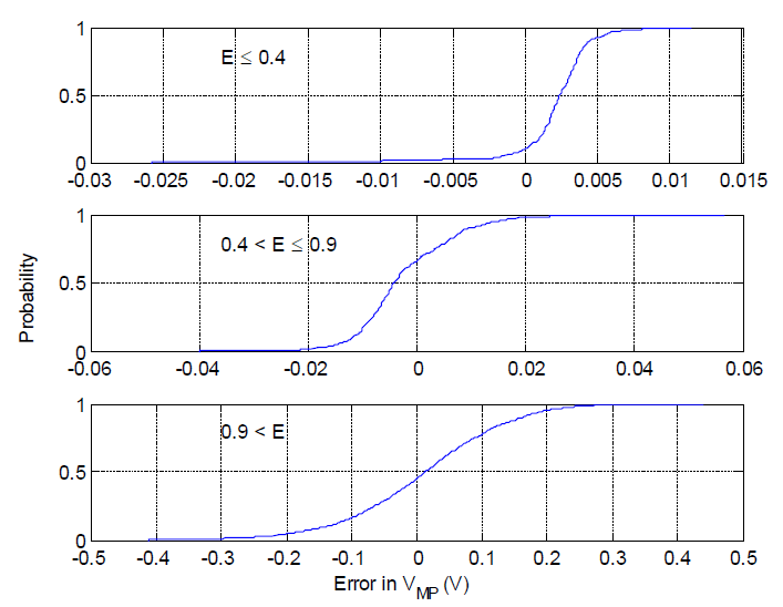
We observe little dependence of the residual for DC current on effective irradiance. By contrast we observe different ranges of the residual for DC voltage for different values of effective irradiance. Due to the correlation between effective irradiance and cell temperature, the residual in DC voltage similarly changes with cell temperature. Consequently, we construct a model for the residuals for DC voltage by partitioning effective irradiance into three intervals:
E1 = {0 ≤ E < 0.4}
E2 = {0.4 ≤ E < 0.9}
E3 = {0.9 ≤ E}
For each interval we construct an empirical distribution for the residual in DC voltage, conditional on that interval. CDFs for these distributions are displayed in the Distributions for residual for DC voltage figure. For DC current we construct one empirical distribution considering the full range of effective irradiance. We sample each distribution independently and assume no temporal correlation between sampled values.
Uncertainty Analysis
Uncertainty Propagation
Conceptually, uncertainty about a model or the model’s inputs implies that the model’s outputs are also uncertain. Here we employ a Monte Carlo technique to generate a sample from the distribution of uncertainty in each model’s output, using the estimated uncertainty in each model’s residuals.
The true value of a model’s output is not known. However, we can obtain a baseline estimate of this unknown value by computing the model’s output using the available model parameters. We also have a distribution for the model’s residuals, which we can randomly sample and combine with the model’s baseline estimate to generate a sample of the true (unknown) model output. For example, consider the POA modeling step. The baseline estimate of POA irradiance,
\(\hat{G}_{POA}(t)\), is known from the POA model. The true value of POA, denoted by
\(G_{POA}(t)\), is unknown, but we have a distribution for the POA residual
\(\delta_{POA}\left (t\mid p_{POA} \right )\)and an equation relating these quantities:
\(\delta_{POA}\left (t\mid p_{POA} \right ) = \cfrac{\hat{G}_{POA}(t)-G_{POA}(t)}{G_{POA}(t)}\)We then regard
\(\delta_{POA}\left (t\mid p_{POA} \right )\)as a random variable, sample a value, and estimate the true (unknown) value for POA irradiance as:
\(G_{POA}(t) = \cfrac{\hat{G}_{POA}(t)}{1+\delta_{POA}\left (t\mid p_{POA} \right )}\)Thus, we obtain a sample for the true value of
\(G_{POA}(t)\). Similar methods are used to generate samples for the true values for other modeled quantities. These samples are passed from one modeling step to the next to compute a sample of DC output from the PV system. Sampling the distributions of model residuals must account for any observed correlations between the residuals and the model’s inputs. For example, the residual in the Isotropic sky diffuse model for estimating POA irradiance from GHI, DNI and DHI exhibits systematic variation over a range of solar zenith angles. Accordingly, we construct uncertainty distributions that account for these correlations.
Calculating PV system output over time inherently involves models with time series inputs, e.g., GHI. Consequently, the sampled model residuals are themselves time series and must reflect appropriate temporal correlations. We address temporal correlations in a rather simplified manner that will tend to overstate the influence of an uncertain time series input on the model’s output. For a small number of distinct conditions, e.g., clear or cloudy skies, morning or afternoon hours, we first judge whether the time series of model residuals exhibits any significant temporal correlation. When a model residual exhibits temporal correlation for a given condition, we assume that time series values remain perfectly correlated until the condition changes. When a model residual shows little or no temporal correlations during a given condition, we randomly and independently sample the model residual at each time step.
Uncertainty Analysis Results

.png)
.png)
.png)
.png)
.png)


We used measured weather data for 2011 (i.e., GHI, DNI, DHI, wind speed and ambient temperature) for Albuquerque, NM, and Golden, CO, and the methods outlined above to generate a sample of size 100 of possible PV system output, i.e., 100 time series of one-minute DC power, with each being one year in length. We reduced these one minute time series to time series of daily DC energy. The Distribution of Daily DC Energy (Isotropic Sky Model) figure shows the results for the SunPowermodule in Albuquerque, NM when using the isotropic sky model. In this figure, one red curve shows the single CDF resulting from the baseline estimate of daily DC energy, with the range of variation in daily energy primarily determined by the variation in daily insolation over the year. The group of blue curves comprises 100 CDFs for daily energy that result from the uncertainty propagation. The separation between the red curve and the group of blue curves indicates a bias on the order of 4% of daily energy that is incurred by using the isotropic sky model in combination with the other component models. The variation among the blue curves represents the range of uncertainty in daily energy that results when uncertainty in each component model is propagated.
.png)
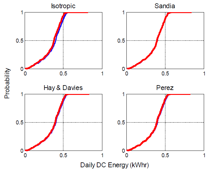
Distributions of Daily DC Energy figure displays the CDFs for daily DC energy, with one plot for each of the POA irradiance models (the remaining models do not vary). In each plot of this figure, one red curve shows the single CDF resulting from the baseline estimate of daily DC energy, with the range of variation in daily energy primarily determined by the variation in daily insolation over the year. Each group of blue curves comprises 100 CDFs for daily energy, one for each sample element. The Distributions of Daily DC Energy figure shows that:
.png)
- For each POA irradiance model, the blue CDFs are tightly grouped, indicating that the overall variation in predicted daily energy is relative small (on the order of 1%).
- For some POA irradiance models (in particular, the isotropic sky and the Hay and Davies models), the group of blue CDFs is offset from the red CDF, indicating that the default parameter values for the POAirradiance models result in POA irradiance predictions that are systematically biased (by upwards of 5%) when compared to onsite measurements.
The SunPower module: Golden, CO, FirstSolar module: Albuquerque, NM, and FirstSolar module: Golden, CO figures show similar results for the SunPower module in Golden, CO, and for the FirstSolarmodule in Albuquerque, NM and Golden CO. These figures confirm that the variation in predicted daily energy is relatively small for either technology and location.
.png)
.png)
.png)
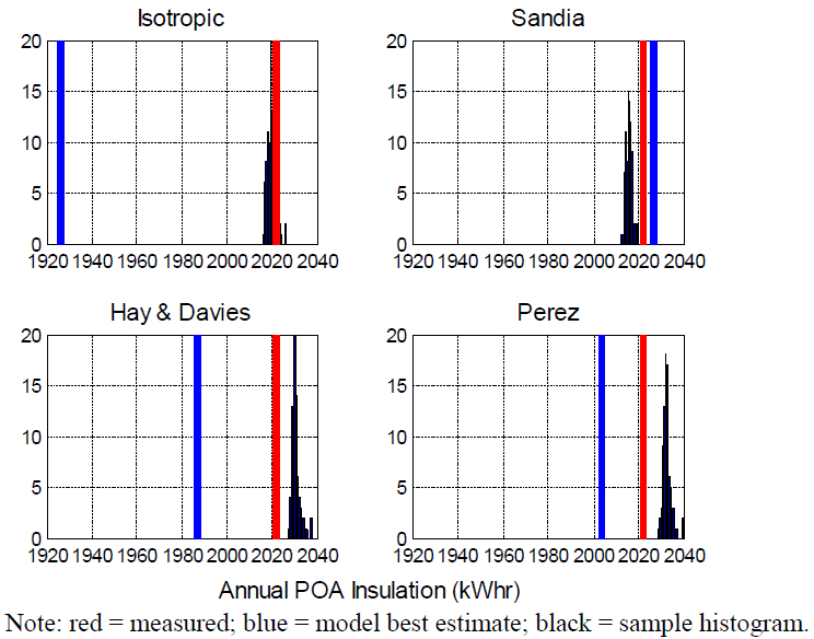
Bias in predicted daily DC energy most likely arises from bias in the POA irradiance models. The Distributions of Annual Insolation: Albuquerque, NM and Distributions of Annual Insolation: Golden, COfigures display the measured annual POA insolation for Albuquerque, NM and Golden CO, respectively, along with the best estimate and the histogram of sampled values for annual POA insolation for each POA irradiance model. The Distributions of Annual Insolation: Albuquerque, NM and Distributions of Annual Insolation: Golden, CO figures confirm that model best estimates can be substantially different from measured values, and that the biases tend to be systematic for each POA irradiance model. These figures also indicate that the sampling strategy for applying residuals to the model best estimate generally obtains a value similar to the measured annual insolation.
.png)
.png)
We explored the origin of the POA model biases by computing the residual in monthly POA insolation. The Residuals for Albuquerque, NM and Residuals for Golden, CO figures display residual as a percent of each month’s measured POA insolation. For Albuquerque, NM, we observe a negative bias on the order of a few percent that is consistent throughout the year; these negative biases are consistent with those found in an analysis of an earlier year. In contrast, for Golden, CO, we see a dramatic change in model bias as the year progresses. We do not know if the late spring residuals in Golden, CO, are a persistent seasonal effect, or an issue with this particular set of measurements. However, we find evidence of biases of similar magnitude, of seasonal variation, and of differences among locations, in other analyses of POA irradiance models[9][10]. Our results and these referenced analyses should be considered as indicating the complexity necessary to consider, if one seeks to improve the accuracy of POA irradiance models.
Sensitivity Analysis
Sensitivity Analysis Methods
Given the results of an uncertainty analysis, a sensitivity analysis examines the relationship between uncertainty in models or model inputs and the resulting uncertainty in the modeling outcomes. The basic model output is DC power at each time step. We quantify uncertainty in DC power in a manner similar to that used to quantify model output uncertainty at each modeling step. We first compute the baseline estimate of DC power by applying a zero residual at each modeling step. We next generate a sample of DC power output by compute the baseline estimate of DC power by applying a zero residual at each modeling step. We then subtract this baseline estimate from each element in the sample for DC power, which results from applying the sampled residual at each modeling step, to obtain a sample of residuals for DC power. We then examine the relationship between the DC power residuals and the various uncertainty distributions for models and for model residuals, by means of correlations and scatterplots.
Formally, we calculate a difference for DC output by ΔPDC(t)
\(\Delta P_{DC}(t) = \hat{P}_{DC}(t)-P_{DC}(t)\)where PDC(t) is the baseline estimate of DC power, obtained by setting
\(\epsilon_{POA}\left (t\mid p_{POA} \right ) = \epsilon_E\left (t\mid p_{E} \right ) = \epsilon_{Tc}\left (t\mid p_{Tc} \right ) = \epsilon_{DC}\left (t\mid p_{VDC} \right )\)We then performed correlations at each time step between ranked values for ΔPDC(t) and ranked values for each of
\(\epsilon_{POA}\left (t\mid p_{POA} \right )\),
\(\epsilon_{E}\left (t\mid p_{E} \right )\),
\(\epsilon_{Tc}\left (t\mid p_{Tc} \right )\)and
\(\epsilon_{DC}\left (t\mid p_{VDC} \right )\). We used stepwise regression reference to build a sequence of regression models for ΔPDC(t) using
\(\epsilon_{POA}\left (t\mid p_{POA} \right )\),
\(\epsilon_{E}\left (t\mid p_{E} \right )\),
\(\epsilon_{Tc}\left (t\mid p_{Tc} \right )\)and
\(\epsilon_{DC}\left (t\mid p_{VDC} \right )\)as predictors. The first model
uses a single predictor; the second model uses the first predictor plus one additional predictor; and so forth. The order in which the predictors are selected for the sequence of regression models indicates the strength of correlation between a predictor and ΔPDC(t).
Intuitively, one expects to see DC power to increase with increasing POA irradiance, increasing effective irradiance, decreasing temperature, and increasing DC voltage or DC current. However, because of the manner in which the residuals are quantified, there is a negative correlation between the sampled values for the residuals (e.g.,
) and the sampled values for true (unknown) value (e.g., GPOA(t). For example, we observe negative correlation between the POA model residual
\(\epsilon_{POA}\left (t\mid p_{POA} \right )\)and the deviation in DC power ΔPDC(t). To permit an intuitive interpretation of our results, we switched the sign of each coefficient in the correlation between ΔPDC(t) and the various model residuals (e.g.,
\(\epsilon_{POA}\left (t\mid p_{POA} \right )\).
Sensitivity Analysis Results
![]()
![]()
![]()
![]()
![]()
The ![]()
The Rank regression coefficients (isotropic sky POA model) figure displays the stepwise rank regression coefficients (SRRCs) for daily energy for the SunPower module and Albuquerque, NM, weather. As a reminder, the predictor variables in the stepwise regression are the model residuals, the predicted variable is the difference between each realization’s power and the power predicted for the base realization, and the signs have been switched on each correlation coefficient. Because model residuals and power are defined at each time step (i.e., at one minute intervals), we reduced each time series of residuals to daily values, as follows:
- For POA irradiance, we summed the model residuals, reasoning that the total residual would correlate with summed differences in DC power output.
- For effective irradiance, we summed the model residuals.
- For cell temperature, we summed the model residuals, reasoning the total temperature difference would predictably correlate with the summed differences in DC power output.
- For DC voltage and DC current, we summed the residuals.
We also added the difference in DC power output to reduce the time series of model outputs to daily values. Regressions are performed between the 100 ranked values for each residual’s daily value and the 100 values for daily energy, first for each day of the calendar year then for each month.
Daily DC Energy
The Rank regression coefficients: SunPower (isotropic sky POA model) figure clearly shows that residuals arising from the isotropic sky POA irradiance model dominate the deviation of modeled power from its baseline value. Residuals arising from the effective irradiance model have a secondary but still significant effect. Residuals arising from the other three models (cell temperature, DC voltage and DC current) are relatively insignificant. The spikes appearing in the various correlation traces correspond to days with highly variable irradiance conditions, when it may be expected that measured air temperature does not instantly and always change with cloud shadows passing over the irradiance sensors, as is anticipated by the models.
The Rank regression coefficients: SunPower (four POA models) shows the stepwise analysis results for daily DC energy for each POAirradiance model for the SunPower module in Albuquerque, NM, and confirms that the residuals arising from the POA irradiance and effective irradiance models are dominant, regardless of which POA irradiance model is used. The Rank regression coefficients: FirstSolar (four POA models) figure displays the stepwise analysis results for daily DC energy for the FirstSolar module in Albuquerque, NM, and confirms that our results are robust for different module technologies. The
Rank regression coefficients: SunPower in Golden, CO, (four POA models) and Rank regression coefficients: FirstSolar in Golden, CO, (four POA models) figures show similar results for Golden, CO, and indicate that our conclusion may not be strongly dependent on location, although a conclusive demonstration would require consideration of more humid and/or cloudy locations. Despite the consideration of only two locations with somewhat similar weather (both are relatively high-altitude, dry locations), we believe that the ranking of the important model residuals will not depend greatly on location.
Monthly DC Energy
Tables below list the stepwise rank correlation coefficients for total monthly (March 2011) DC energy for the SunPower and FirstSolar modules, respectively, where the monthly residuals for each predictor were computed similar to the calculation of the daily predictors. The consistent ranking of the predictors among the four POA and the trends in R2 values both confirm the dominance of the POA and effective irradiance models.
The Rank regression coefficients: SunPower (monthly) and Rank regression coefficients: SunPower (monthly) figures show the R2 values achieved as each variable is added to the stepwise regression model for monthly energy for the SunPower module in Albuquerque, NM, and Golden, CO, respectively. Except for May, 2011, in Golden, CO, the complete stepwise model achieves a relatively high R2 and the relative importance of the various model residuals is consistent across the year for both locations. These results indicate the robustness of our sensitivity analysis results.
Dependence on ground albedo value
![]()
![]()

![]()
The sensitivity analysis indicates that uncertainty in predicted energy yield arises primarily from uncertainty in the POA irradiance models. We characterized uncertainty in these models in terms of model residuals quantified by comparing model predictions with measured POA irradiance. However, we did not vary each model’s parameters; specifically, each POA irradiance model used the same assumed value for albedo, 0.2. Here, we consider whether the conclusions of our sensitivity analysis depend on this parameter value.
As described in POA Irradiance Chapter, POA irradiance GPOA is modeled as the sum of three components – beam irradiance Eb, ground-reflected diffuse irradiance Ediff,g and sky diffuse irradiance Ediff,sky
\(G_{POA} = E_b+E_{diff,g}+E_{diff,sky}\)The four POA irradiance models considered simulate only the sky diffuse irradiance Ediff,sky. All POA irradiance models use the same expression for beam irradiance, i.e.,:
\(E_b = DNI\times cos(AOI)\)and the same expression for ground reflected diffuse irradiance:
\(E_{diff,g} = GHI\times a \times \cfrac{1-cos(A)}{2}\)where A is the tilt angle of the module towards the equator (assumed constant and precisely known) and a is the value for ground albedo. Thus, uncertainty in POA diffuse irradiance is characterized by uncertainty in the sky diffuse irradiance model (which we quantified by empirical distributions of each model’s residual) and by uncertainty in the albedo a.
| Hay and Davies model | Isotropic model | ||||
|---|---|---|---|---|---|
| Variable | SRRC | R2 | Variable | SRRC | R2 |
| POA | 0.837419 | 0.73584 | POA | 0.870833 | 0.794909 |
| Ee | 0.503523 | 0.986931 | Ee | 0.443536 | 0.989552 |
| Tc | -0.04452 | 0.988952 | Tc | -0.03997 | 0.99117 |
| Imp | 0.013275 | 0.989113 | Imp | 0.010019 | 0.991263 |
| Vmp | 0.003754 | 0.989126 | Vmp | 0.001764 | 0.991266 |
| Sandia model | Perez model | ||||
| Variable | SRRC | R2 | Variable | SRRC | R2 |
| POA | 0.866062 | 0.785993 | POA | 0.816113 | 0.710919 |
| Ee | 0.453124 | 0.988824 | Ee | 0.526815 | 0.985536 |
| Tc | -0.04364 | 0.990752 | Tc | -0.04823 | 0.987897 |
| Imp | 0.012462 | 0.990894 | Imp | 0.017454 | 0.988166 |
| Vmp | 0.002459 | 0.9909 | Vmp | 0.007244 | 0.988215 |
| Hay and Davies model | Isotropic model | ||||
|---|---|---|---|---|---|
| Variable | SRRC | R2 | Variable | SRRC | R2 |
| POA | 0.84322 | 0.746561 | POA | 0.874678 | 0.804208 |
| Ee | 0.496835 | 0.987192 | Ee | 0.437243 | 0.990075 |
| Imp | 0.045569 | 0.988945 | Imp | 0.038176 | 0.991271 |
| Tc | -0.03552 | 0.990229 | Tc | -0.03184 | 0.992293 |
| Vmp | 0.010156 | 0.990323 | Vmp | 0.006724 | 0.992334 |
| Sandia model | Perez model | ||||
| Variable | SRRC | R2 | Variable | SRRC | R2 |
| POA | 0.869865 | 0.795624 | POA | 0.822758 | 0.722397 |
| Ee | 0.446909 | 0.989323 | Ee | 0.520405 | 0.985827 |
| Imp | 0.0419 | 0.990752 | Imp | 0.048661 | 0.987799 |
| Tc | -0.03539 | 0.992014 | Tc | -0.03887 | 0.989327 |
| Vmp | 0.007499 | 0.992065 | Vmp | 0.010664 | 0.989431 |
Our uncertainty quantification for POA irradiance, uncertainty analysis, and sensitivity analysis are all conditional on a constant, assumed value a = 0.2, which is typical for PV systems[8]. We repeated the uncertainty and sensitivity analysis using two different assumed values, 0.1 and 0.3, to determine whether our conclusions depend on the assumed albedo value.
The Total annual POA insolation for different albedo values figure displays total annual POA insolation predicted by the XXX model for Albuquerque, NM, for different values of albedo (0.1, 0.2, and 0.3). For comparison, total annual measured POA insolation is shown as a red line in this figure. For the various albedo values the difference in predicted POA insolation is small, roughly 1% of the total annual amount. Differences among predicted POA insolation values are also small for the other three models.
The Rank regression coefficients: SunPower (Perez model) figure displays stepwise rank regression coefficients for daily DC energy for the SunPower module using measured weather data from Golden, CO, the Perez sky diffuse model, and the different albedo values. There is little difference among the plots, confirming that the conclusions of the sensitivity analysis do not depend on the albedo value. Similar results are observed for other POA irradiance models, and for the FirstSolar module and for Albuquerque, NM.
Conclusions
We report an uncertainty and sensitivity analysis for modeling DC energy from photovoltaic systems. We considered two systems, each comprising a single module using either crystalline silicon or CdTe cells, and located either at Albuquerque, NM, or Golden, CO. We quantified uncertainty in the following modeling steps:
- Translation from measured GHI, DNI and DHI to POA irradiance;
- Estimation of effective irradiance (i.e., irradiance converted to electrical current);
- Prediction of cell temperature from measured air temperature and wind speed;
- Production of DC voltage and current from the module.
Due to the complexity and correlations among each model’s parameters, we adopt an approach where we characterize the uncertainty in a model’s output by quantifying the distribution of each model’s residual, i.e., the difference between the model’s prediction and the true value, rather than the traditional approach of quantifying uncertainty in each input parameter.
We found that the overall uncertainty in predicted PV system output, i.e., daily energy, to be relatively small, on the order of 1%. Four alternative models were considered for the POA irradiance modeling step; we did not find the choice of one of these models to be of great significance. However, we found that all POA irradiance models exhibited a systematic bias of upwards of 5% that depends on location, and that this bias translates proportionally to differences in predicted energy.
Sensitivity analyses relate uncertainty in the PV system output to uncertainty arising from each model. We found that the errors arising from the POA irradiance and the effective irradiance models to be the dominant contributors to uncertainty in daily energy, for either technology or location considered. This analysis indicates that efforts to reduce the uncertainty in PV system output should focus on improvements to the POA and effective irradiance models.
References
- ↑ Sandia, Uncertainty and Sensitivity Analysis for Photovoltaic System Modeling, December 2013, [Online]. Available: http://energy.sandia.gov/wp/wp-content/gallery/uploads/SAND2013-10358_Hansen-Uncertainty.pdf. [Accessed April 2014].
- ↑ Whitfield, K. and C.R. Osterwald, Procedure for determining the uncertainty of photovoltaic module outdoor electrical performance. Progress in Photovoltaics: Research and Applications, 2001. 9(2): p. 87-102.
- ↑ Dominé, D., et al. Uncertainties of PV Module – Long-term Outdoor Testing. in 25th PVSEC, 2012. Valencia, Spain.
- ↑ Helton, J.C., J.D. Johnson, and W.L. Oberkampf, An exploration of alternative approaches to the representation of uncertainty in model predictions. Reliability Engineering & System Safety, 2004. 85(1–3): p. 39-71.
- ↑ 5.0 5.1 5.2 Hay, J.E. and J.A. Davies. Calculations of the solar radiation incident on an inclined surface. in First Canadian Solar Radiation Data Workshop, 59, 1980. Ministry of Supply and Services, Canada.
- ↑ 6.0 6.1 Hughes, G.W., Engineering Astronomy, 1985, Sandia National Laboratories.
- ↑ Kasten, F. and A.T. Young, Revised optical air mass tables and approximation formula. Applied Optics, 1989. 28(22): p. 4735-4738.
- ↑ 8.0 8.1 Lorenzo, E., Energy Collected and Delivered by PV Modules, in Handbook of Photovoltaic Science and Engineering, A. Luque, Hegedus, S., Editor. 2011, John Wiley and Sons.
- ↑ Serra, E.B., M.G. Gómez, and M. Hartung. Evaluation of the Energy Yield Prediction Error Depending on the Methodology to Estimate Global Tilted Irradiance from Measured Global Horizontal Irradiance. in 39th IEEE PVSC, 2013. Tampa, FL.
- ↑ Gueymard, C.A., Direct and indirect uncertainties in the prediction of tilted irradiance for solar engineering applications. Solar Energy, 2009. 83(3): p. 432-444.